Introduction Multivariate procedures in R Until version 2.1.0, R - PowerPoint PPT Presentation
Introduction Multivariate procedures in R Until version 2.1.0, R had limited support for multivariate tests Repeated measurements similar to those in SAS/SPSS Peter Dalgaard seems to have some value Department of Biostatistics
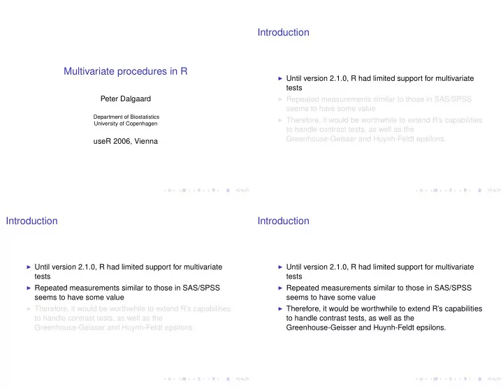
Introduction Multivariate procedures in R ◮ Until version 2.1.0, R had limited support for multivariate tests ◮ Repeated measurements similar to those in SAS/SPSS Peter Dalgaard seems to have some value Department of Biostatistics ◮ Therefore, it would be worthwhile to extend R’s capabilities University of Copenhagen to handle contrast tests, as well as the Greenhouse-Geisser and Huynh-Feldt epsilons. useR 2006, Vienna Introduction Introduction ◮ Until version 2.1.0, R had limited support for multivariate ◮ Until version 2.1.0, R had limited support for multivariate tests tests ◮ Repeated measurements similar to those in SAS/SPSS ◮ Repeated measurements similar to those in SAS/SPSS seems to have some value seems to have some value ◮ Therefore, it would be worthwhile to extend R’s capabilities ◮ Therefore, it would be worthwhile to extend R’s capabilities to handle contrast tests, as well as the to handle contrast tests, as well as the Greenhouse-Geisser and Huynh-Feldt epsilons. Greenhouse-Geisser and Huynh-Feldt epsilons.
Theoretical Setting Theoretical Setting Multivariate normal model: Multivariate normal model: Y ∼ N (Ξ B , I ⊗ Σ) Y ∼ N (Ξ B , I ⊗ Σ) ◮ Y is N × p matrix ◮ Y is N × p matrix ◮ Rows y i of Y are independent with same covariance Σ ◮ Rows y i of Y are independent with same covariance Σ ◮ Ξ is a design matrix (sorry, I used X for other purposes. . . ) ◮ Ξ is a design matrix (sorry, I used X for other purposes. . . ) ◮ Same linear model for all p coordinates (separate ◮ Same linear model for all p coordinates (separate parameters in columns of B ) parameters in columns of B ) ◮ For convenience, we refer to the rows of Y as “subjects”. ◮ For convenience, we refer to the rows of Y as “subjects”. Theoretical Setting Theoretical Setting Multivariate normal model: Multivariate normal model: Y ∼ N (Ξ B , I ⊗ Σ) Y ∼ N (Ξ B , I ⊗ Σ) ◮ Y is N × p matrix ◮ Y is N × p matrix ◮ Rows y i of Y are independent with same covariance Σ ◮ Rows y i of Y are independent with same covariance Σ ◮ Ξ is a design matrix (sorry, I used X for other purposes. . . ) ◮ Ξ is a design matrix (sorry, I used X for other purposes. . . ) ◮ Same linear model for all p coordinates (separate ◮ Same linear model for all p coordinates (separate parameters in columns of B ) parameters in columns of B ) ◮ For convenience, we refer to the rows of Y as “subjects”. ◮ For convenience, we refer to the rows of Y as “subjects”.
Theoretical Setting Standard test procedures Multivariate normal model: 1. Reduce mean value structure, same for all coordinates: Look at Y ∼ N (Ξ B , I ⊗ Σ) MS − 1 res MS eff (generalized F test) Multiple ways of turning this matrix into a test statistic: ◮ Y is N × p matrix Wilks’ Λ (LRT), Pillai trace, Hotelling-Lawley, Roy’s greatest ◮ Rows y i of Y are independent with same covariance Σ root. All are different combinations of the eigenvalues. ◮ Ξ is a design matrix (sorry, I used X for other purposes. . . ) 2. Test that Σ is proportional to Σ 0 (usually I ): Mauchly’s test ◮ Same linear model for all p coordinates (separate of sphericity. parameters in columns of B ) 3. Test mean value structure, assuming that the variance is ◮ For convenience, we refer to the rows of Y as “subjects”. known up to a constant: This is GLS and leads to an F test Standard test procedures Standard test procedures 1. Reduce mean value structure, same for all coordinates: 1. Reduce mean value structure, same for all coordinates: Look at Look at MS − 1 MS − 1 res MS eff res MS eff (generalized F test) (generalized F test) Multiple ways of turning this matrix into a test statistic: Multiple ways of turning this matrix into a test statistic: Wilks’ Λ (LRT), Pillai trace, Hotelling-Lawley, Roy’s greatest Wilks’ Λ (LRT), Pillai trace, Hotelling-Lawley, Roy’s greatest root. All are different combinations of the eigenvalues. root. All are different combinations of the eigenvalues. 2. Test that Σ is proportional to Σ 0 (usually I ): Mauchly’s test 2. Test that Σ is proportional to Σ 0 (usually I ): Mauchly’s test of sphericity. of sphericity. 3. Test mean value structure, assuming that the variance is 3. Test mean value structure, assuming that the variance is known up to a constant: This is GLS and leads to an F test known up to a constant: This is GLS and leads to an F test
Within-Subject Contrasts Within-Subject Contrasts ◮ You often need to consider a transformation of responses ◮ You often need to consider a transformation of responses ◮ If coordinates are repeated measures, you might wish to ◮ If coordinates are repeated measures, you might wish to test for “no change over time” or “same changes over time test for “no change over time” or “same changes over time in different groups” (profile analysis). This leads to the in different groups” (profile analysis). This leads to the analysis of within-subject contrasts. analysis of within-subject contrasts. ◮ Also, in a mixed-model setting, the subject effect will ◮ Also, in a mixed-model setting, the subject effect will cancel out in the contrasts, whose distribution may then be cancel out in the contrasts, whose distribution may then be assumed to satisfy a sphericity condition. assumed to satisfy a sphericity condition. Within-Subject Contrasts More General Transformations ◮ Similar notions carry over to more elaborate within-subject ◮ You often need to consider a transformation of responses designs ◮ If coordinates are repeated measures, you might wish to ◮ E.g. a two-way layout and then look at test for “no change over time” or “same changes over time ◮ Contrasts between row means in different groups” (profile analysis). This leads to the ◮ Contrasts between column means analysis of within-subject contrasts. ◮ Interaction contrasts ◮ Also, in a mixed-model setting, the subject effect will ◮ Variance component model with “all terms containing cancel out in the contrasts, whose distribution may then be subject considered random” implies sphericity of each of assumed to satisfy a sphericity condition. the above (with different constants)
More General Transformations More General Transformations ◮ Similar notions carry over to more elaborate within-subject ◮ Similar notions carry over to more elaborate within-subject designs designs ◮ E.g. a two-way layout and then look at ◮ E.g. a two-way layout and then look at ◮ Contrasts between row means ◮ Contrasts between row means ◮ Contrasts between column means ◮ Contrasts between column means ◮ Interaction contrasts ◮ Interaction contrasts ◮ Variance component model with “all terms containing ◮ Variance component model with “all terms containing subject considered random” implies sphericity of each of subject considered random” implies sphericity of each of the above (with different constants) the above (with different constants) More General Transformations More General Transformations ◮ Similar notions carry over to more elaborate within-subject ◮ Similar notions carry over to more elaborate within-subject designs designs ◮ E.g. a two-way layout and then look at ◮ E.g. a two-way layout and then look at ◮ Contrasts between row means ◮ Contrasts between row means ◮ Contrasts between column means ◮ Contrasts between column means ◮ Interaction contrasts ◮ Interaction contrasts ◮ Variance component model with “all terms containing ◮ Variance component model with “all terms containing subject considered random” implies sphericity of each of subject considered random” implies sphericity of each of the above (with different constants) the above (with different constants)
Recommend
More recommend
Explore More Topics
Stay informed with curated content and fresh updates.
