Interprocedural Analysis and Abstract Interpretation cs6463 1 - PowerPoint PPT Presentation

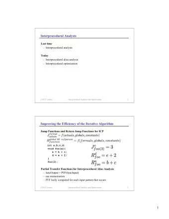
Interprocedural Analysis and Abstract Interpretation cs6463 1

Outline  Interprocedural analysis  control-flow graph  MVP: “Meet” over Valid Paths  Making context explicit  Context based on call-strings  Context based on assumption sets  Abstract interpretation cs6463 2

Control-flow graph for a whole program At each function definition proc p(x)  Create two special CFG nodes:   init(p) and final(p) Build CFG for the function body   Use init(p) as the function entry node  Connect every return node to final(p) At each function call to p(x) with  Split the original function call into two stmts   Enter p(x) (before making the call) and exit p(x) (after the call exits) Connect enter p(x) ->init(p), final(p) -> exit p(x)  Connect enter p(x) -> exit p(x) to allow the flow of extra context info  Three kinds of CFG edges  Intra-procedural: internal control-flow within a procedure  Procedure calls: from enter p(x) to init(p)  Procedure returns: from final(p) to exit p(x)  cs6463 3

Interprocedural CFG Example B0: init(fib) int fib(int z) { if (z < 3) then return 1; B1: if (z < 3) else return fib(z-1) + fib(z-2); } B2: enter fib(z-1) Main program: return fib(15); B5: return 1 B3:t1=exit fib(z-1) A0:enter fib(15) enter fib(z-2) B4:t2=exit fib(z-2) return t1+t2; A1: t = exit fib(15) B6: final(fib)  Problem: matching between function calls and returns cs6463 4

Extending monotone frameworks  Monotone frameworks consists of  A complete lattice (L, ≤ ) that satisfies the Ascending Chain Condition  A set F of monotone transfer functions from L to L that  contains the identity function and  is closed under function composition  Transfer functions for procedure definitions  For simplicity, both init(p) and final(p) have identity transfer functions  Transfer functions for procedure calls  For procedure entry: assign values to formal parameters  For procedure exit: assign return values to outside cs6463 5

Problem: calling context upon return B0: init(fib) int fib(int z) { if (z < 3) then return 1; B1: if (z < 3) else return fib(z-1) + fib(z-2); } B2: enter fib(z-1) Main program: return fib(15); B5: return 1 B3:t1=exit fib(z-1) A0:enter fib(15) enter fib(z-2) B4:t2=exit fib(z-2) return t1+t2; A1: t = exit fib(15) B6: final(fib) Matching between function calls and returns   Calculating solutions on non-existing paths could seriously detriment precision  E.g. enter fib(z-2) -> init(fib) -> … -> exit fib(z-1) -> … cs6463 6

MVP: “Meet” over Valid Paths  Problem: matching procedure entries and exits (function calls and returns)  A complete path must  Have proper nesting of procedure entries and exits  A procedure always return to the point immediately after it is called  A valid path must  Start at the entry node of the main program  All the procedure exits match the corresponding entries  Some procedures may be entered but not yet exited  The MVP solution  At each program point t, the solution for t is  MVP(t) = Λ { sol(p) : p is a valid path to t } cs6463 7

Making Context Explicit  Context sensitive analysis  Maintain separate solutions for different callers of a function  Extending the monotone framework  Starting point (context-insensitive)  A complete lattice (L, ≤ ) that satisfies the Ascending Chain Condition  L = Power(D) where D is the domain of each solution  A set F of monotone transfer functions from L to L  Extension  L = Power( D * C), where C includes all calling contexts  F = L -> L, a separate sub-solution is calculated for each calling context  F (procedure entry) : attach caller info. to incoming solution  F (procedure exit): match caller info, eliminate solution for invalid paths cs6463 8

Different Kinds of Context  Call strings --- contexts based on control flow  Remember a list of procedure calls leading to the current program point  Call strings of unbounded length --- remember all the preceding calls  Call strings of bounded length (k) --- remember only the last k calls  Assumption sets --- contexts based on data flow  Assumption sets  Use the solution before entering proc p(x) as calling context (e.g., each context makes distinct presumptions about values of function parameters)  Large vs. small assumption sets  How large is the context: use the entire solution or pick a single constraint from the solution cs6463 9

Example Context-sensitive Analysis B0: init(fib) int fib(int z) { if (z < 3) then return 1; B1: if (z < 3) else return fib(z-1) + fib(z-2); } B2: enter fib(z-1) Main program: return fib(15); B5: return 1 B3:t1=exit fib(z-1) A0:enter fib(15) enter fib(z-2) B4:t2=exit fib(z-2) return t1+t2; A1: t = exit fib(15) B6: final(fib)  Range analysis: for each variable reference x, is its value >= or <= a constant value? (i.e, x >= x1; z<=n2)? cs6463 10

Example Range Analysis Variables: x,z, t1, t2, fib, t; Contexts: A0, B2, B3,none; Domain: Variables * (<=n, =n, >=n,?,any) (none) (none) (none) (none) A0 (none, (A0,z=15) (B2/B3, (A0,z=15)(B2,z>=2) (A0,z=15)(B2,z>=2) B0 z=?) z=?) (B3,z>=1) (B3,z>=1) (none, (A0,z=15) (B2/B3, (A0,z=15)(B2,z>=2) B1 (A0,z=15)(B2,z>=2) z=?) z=?) (B3,z>=1) (B3,z>=1) (none, (A0,z=15) (B2/B3, (A0,z=15)(B2/B3,z> (A0,z=15)(B2/B3,z>= B2 z=?) z>=3) =3) 3) (none, (A0,z=15,t1=?) (A0,z=15,t1=1) (A0,z=15,t1>=1) B3 z/t1=?) (B2/B3,z>=3,t1=?) (B2/B3,z>=3,t1=1) (B2/B3,z>=3,t1>=1) (none, (A0,z=15,t1/t2=?)(B (A0,z=15,t1/t2=1)(B (A0,z=15,t1/t2>=1)(B B4 z/t1/t2=?) 2/B3,z>=3,t1/t2=?) 2/B3,z>=3,t1/t2=1) 2/B3,z>=3,t1/t2>=1) (none, (B2/B3,z<=2) (B2,z=2) (B3,z<=2) (B2,z=2) (B3,z<=2) B5 z=?) (none,z/fib (A0,z=15,fib=?)(B2/ (A0,z=15,fib>=1)(B2 (A0,z=15,fib>=1)(B2/ B6 =?) B3,z=any,fib=1) /B3,z=any,fib>=1) B3,z=any,fib>=1) A1 (none,t=?) (none,t=?) (none,t >=1) (none,t>=1) cs6463 11

Foundations of Abstract Interpretation  Definition from Wikipedia  abstract interpretation is a theory of sound approximation of the semantics of computer programs. It can be viewed as a partial execution of a computer program without performing all the calculations .  Outline  Monotone frameworks  A complete lattice (L, ≤ ) that satisfies the Ascending Chain Condition  A set F of monotone transfer functions from L to L that  contains the identity function and  is closed under function composition  Galois connections, closures,and Moore families  Soundness and completeness of operations on abstract data  Soundness and completeness of execution trace computation cs6463 12

Galois Connections  Two complete lattices  C: the “concrete” (execution) data  The execution of the entire program  Infinite and impossible to model precisely  A: the “abstract” (execution) data  Properties (abstractions) of the “concrete” data  The solution space (domain) of static program analysis  For complete lattices C and A, a Galois connection is  A pair of monotonic functions, α : C->A, γ : A -> C  For all a ∈ A and c ∈ C: c ≤ γ ( α (c)) and α ( γ (a)) ≤ a  Is Written as C< α , γ >A A C cs6463 13

Galois Connections (2)  γ and α are inverse maps of each other ’ s image γ  For all c ∈ γ (A),c= γ ( α (c)); for all {1,2,3,4,…} a ∈ α (C),a= α ( γ (a)) all  The maps α are {1,3,5,7…} “homomorphism” mappings even odd between C and A {1,2,3} {1,3,5} α  Galois connections are closed {2,4} under none {1}  Composition, product, and so {} on  Each instruction performs an action f: C->C  Can use α and γ to define an abstract transfer function f#: A->A for each f: C->C cs6463 14

Closure Maps  For C< α , γ >A, it is common that {1,2,3,4,…} α all A ⊆ C. This means A embeds {1,3,5,7…} into C as a sub-lattice even odd  A ’ s elements name {1,2,3} {1,3,5} γ distinguished sets in C {2,4} none {1}  A closure map defines the embedding of A within C. {} Definition: ρ : C->C is a closure 1) Every Galois connection, map if it is C < α , γ >A defines a closure  Monotonic: ∀ c1,c2 ∈ C, c1 ≤ c2 => ρ (c1) ≤ ρ (c2); map α • γ ; Every closure map, ρ : C-  extensive: ∀ c ∈ C, c ≤ ρ (c); 2)  idempotent: ∀ c ∈ C, ρ ( ρ (c))= >C,defines the Galois ρ (c) (i.e. ρ * ρ = ρ ) connection, C< ρ ,id> ρ (C) . cs6463 15

Moore Families  Given C, can we define a closure map on it by choosing some elements of C?  Yes , if the elements we select are closed under greatest-lower-bounds (meet) operation  That is, the new set of elements forms a complete lattice  Definition: M ⊆ C is a Moore family iff for all S ⊆ M, (^S) ∈ M.  We can define a closure map as ρ (c)=^{c ’ ∈ M | c ≤ c ’ }.  That is, we map each element in C to the closest abstraction (approximation) in M  For each closure map, ρ :C->C, its image, ρ (C), is a Moore family. Given C, we can define an abstract interpretation by selecting some M ⊆ C that is a Moore family cs6463 16