Interpolation Introduction 1. For analyzing functions f ( x ) , say - PowerPoint PPT Presentation

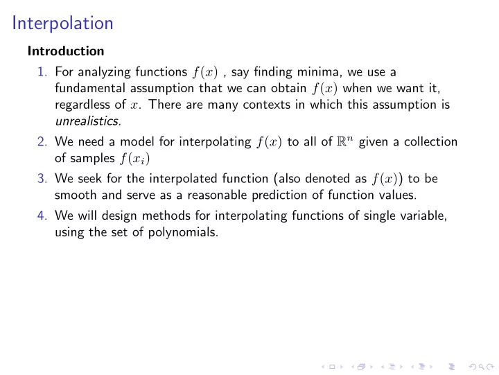
Interpolation Introduction 1. For analyzing functions f ( x ) , say finding minima, we use a fundamental assumption that we can obtain f ( x ) when we want it, regardless of x . There are many contexts in which this assumption is unrealistics. 2. We need a model for interpolating f ( x ) to all of R n given a collection of samples f ( x i ) 3. We seek for the interpolated function (also denoted as f ( x ) ) to be smooth and serve as a reasonable prediction of function values. 4. We will design methods for interpolating functions of single variable, using the set of polynomials.

Interpolation Polynomial representation in a basis: f ( x ) = a 1 φ 1 ( x ) + a 2 φ 2 ( x ) + · · · + a k φ k ( x ) where { φ 1 ( x ) , φ 2 ( x ) , . . . , φ k ( x ) } is a basis: 1. Monomial basis: φ i ( x ) = x i − 1

Interpolation 2. Lagrange basis � j � = i ( x − x j ) � φ i ( x ) = j � = i ( x i − x j ) where { x 1 , x 2 , . . . , x k } are prescribed distinct points. Note that � 1 when ℓ = i φ i ( x ℓ ) = 0 otherwise φ 2 φ 3 φ 4 φ 1 1 0 2 3 4

Interpolation 3. Newton basis i − 1 � φ i ( x ) = ( x − x j ) with φ 1 ( x ) ≡ 1 , j =1 where { x 1 , x 2 , . . . , x k } are prescribed distinct points. Note that φ i ( x ℓ ) = 0 for all ℓ < i . 10 ψ 4 ψ 3 ψ 2 ψ 1 0 2 3 4

Interpolation Polynomial interpolation: Given a set of k points ( x i , y i ) , with the assumption x i � = x j . Find a polynomial f ( x ) of degree k − 1 such that f ( x i ) = y i .

Interpolation 1. Interpolating polynomial in monomial basis f ( x ) = a 1 + a 2 x + a 3 x 2 + · · · + a k x k − 1 where a 1 , a 2 , . . . , a k are determined by the Vandermonde linear system:       x k − 1 x 2 1 x 1 · · · a 1 y 1 1 1       x 2 x k − 1 1 x 2 · · · a 2 y 2       2 2      =   . . . . . . . . . . . . . .      . . . . . . . x 2 x k − 1 a k y k 1 x k · · · k k 2. Interpolating polynomial in Lagrange basis f ( x ) = y 1 φ 1 ( x ) + y 2 φ 2 ( x ) + · · · + y k φ k ( x )

Interpolation 3. Interpolating polynomial in Newton basis f ( x ) = a 1 φ 1 ( x ) + a 2 φ 2 ( x ) + · · · + a k φ k ( x ) where a 1 , a 2 , . . . , a k are determined by the following triangular systems:       1 a 1 y 1       1 φ 2 ( x 2 ) a 2 y 2        =       . . . . ... . . . .      . . . . 1 φ 2 ( x k ) · · · φ k ( x k ) a k y k

Interpolation Remarks 1. The Verdermonde system could be poor conditioned and unstable. 2. Computing f ( x ) in Lagrange basis takes O ( k 2 ) time, constrastingly, computing f ( x ) in monomial basis takes only O ( k ) by Horner’s rule. 3. f ( x ) in Newton basis attempts to compromise between the numerical quality of the monomial basis and the efficiency of the Lagrange basis. Examples ◮ interpeg1.m ◮ interpeg2.m ◮ interpeg3.m

Piecewise interpolation 1. So far, we have constructed interpolation bases defined on all of R . 2. When the number k of data points becomes large, many degeneracies apparent. Mostly noticble, the polynomial interpolation is nonlocal , changing any single value y i can change the behavior of f ( x ) for all x , even those that are far away from x i . This property is undersiable from most applications. 3. A solution to avoid such drawback is to design a set of base functions φ i ( x ) of the property of compact support : A function g ( x ) has compact support if there exists a constant c ∈ R such that g ( x ) = 0 for any x with � x � 2 > c . 4. Piecewise formulas provide one technique for constructing interpolatory bases with compact support.

Piecewise interpolation Piecewise constant interpolation: 1. Order the data points such that x 1 < x 2 < · · · < x k 2. For i = 1 , 2 , . . . , k , define the basis � when x i − 1 + x i ≤ x < x i + x i +1 1 φ i ( x ) = 2 2 0 otherwise 3. Piecewise constant interpolation k � f ( x ) = y i φ i ( x ) i =1 4. discontinuous!

Piecewise interpolation Piecewise linear interpolation : 1. Order the data points such that x 1 < x 2 < · · · < x k 2. Define the basis (”hat functions”)  x − x i − 1  when x i − 1 < x ≤ x i  x i − x i − 1 x i +1 − x φ i ( x ) = when x i < x ≤ x i +1  x i +1 − x i  0 otherwise for i = 2 , . . . , k − 1 with the boundary “half-hat” basis φ 1 ( x ) and φ k ( x ) . 3. Piecewise linear interpolation k � f ( x ) = y i φ i ( x ) i =1 4. Continuous, but non-smooth. 5. Smooth piecewise high-degree polynomial interpolation – “splines”

Piecewise interpolation Piecewise constant Piecewise linear P i e c e w i s e c o n s t a n t P i e c e w i s e l i n e a r

Theory of interpolation 1. Linear algebra of functions 2. Error bound of piecewise interpolations

Theory of interpolation Linear algebra of functions 1. There are other bases (beyond monomials, Lagranges and Newtons) for the set of functions f . 2. Inner product of functions f and g : � b � f, g � w = w ( x ) f ( x ) g ( x ) dx a and � � f � = � f, f � w where w ( x ) is a given positive (weighting) function.

Theory of interpolation 3. Lagendre polynomials Let a = − 1 , b = 1 and w ( x ) = 1 , applying Gram-Schmidt process to the monomial basis { 1 , x, x 2 , x 3 , . . . } , we generate the Lagendre basis of polynomials: P 0 ( x ) = 1 P 1 ( x ) = x P 2 ( x ) = 1 2(3 x 2 − 1) P 3 ( x ) = 1 2(5 x 3 − 3 x ) , . . . where { P i ( x ) } are orthogonal.

Theory of interpolation 4. An application of Lagendre polynomials: Least squares function approximation (not interpolation) n n � � a ∗ min a i � f − a i P i ( x ) � = � f − i P i ( x ) � i =1 i =1 where i = � f, P i � a ∗ � P i , P i � . Note that we need intergration here, numerical integration to be covered later.

Theory of interpolation 5. Chebyshev polynomials 1 Let a = − 1 , b = 1 and w ( x ) = 1 − x 2 , applying √ Gram-Schmidt process to the monomial basis { 1 , x, x 2 , x 3 , . . . } , we generate the Chebyshev basis of polynomials: T 0 ( x ) = 1 T 1 ( x ) = x T 2 ( x ) = 2 x 2 − 1 T 3 ( x ) = 4 x 3 − 3 x, . . . where { T i ( x ) } are orthogonal.

Theory of interpolation 6. Surprising properties of Chebyshev polynomials (a) Three-term recurrence T k +1 = 2 xT k ( x ) − T k − 1 ( x ) with T 0 ( x ) = 1 and T 1 ( x ) = x . (b) T k ( x ) = cos( k arccos( x )) ◮ ... 7. Chebyshev polynomials play important role in modern numerical algorithms for solving very large scale linear systems and eigenvalue and singular value problems!

Theory of interpolation Error bound of piecewise interpolations 1. Consider the approximation of a function f ( x ) with a polynomial of degree n on an interval [ a, b ] . Define ∆ = b − a 2. Piecewise constant interpolation If we approximate f ( x ) with a constant c = f ( a + b 2 ) , as in piecewise constant interpolation, and assume that | f ′ ( x ) | ≤ M for all x ∈ [ a, b ] , then x ∈ [ a,b ] | f ( x ) − c | ≤ M∆x = O ( ∆x ) max

Theory of interpolation 3. Piecewise linear interpolation Approximate f ( x ) with f ( x ) = f ( a ) b − x b − a + f ( b ) x − a � b − a . By the Taylor series f ( a ) = f ( x ) + ( a − x ) f ′ ( x ) + · · · f ( b ) = f ( x ) + ( b − x ) f ′ ( x ) + · · · we have f ( x ) = f ( x ) + 1 � 2( x − a )( x − b ) f ′′ ( x ) + O (( ∆x ) 3 ) . Therefore, the error = O ( ∆x 2 ) assuming f ′′ ( x ) is bounded. Note that | x − a | | x − b | ≤ 1 2 ( ∆x ) 2 .