interpolation L. Olson Department of Computer Science University - PowerPoint PPT Presentation
interpolation L. Olson Department of Computer Science University of Illinois at Urbana-Champaign 1 semester plan Tu Nov 10 Least-squares and error Th Nov 12 Case Study: Cancer Analysis Tu Nov 17 Building a basis for approximation
interpolation L. Olson Department of Computer Science University of Illinois at Urbana-Champaign 1
semester plan Tu Nov 10 Least-squares and error Th Nov 12 Case Study: Cancer Analysis Tu Nov 17 Building a basis for approximation (interpolation) Th Nov 19 non-linear Least-squares Tu Dec 01 non-linear Least-squares Th Dec 03 optimization methods Tu Dec 08 Elements of Simulation + Review 2
interpolation Today’s ojbectives: 1. Take a few points and interpolate instead of fit 2. Write the interpolant as a combination of *basis* functions 3. Implemente interpolation with several types of basis functions 4. Construct interpolation through a linear algebra problem 3
interpolation: introduction Objective Approximate an unknown function f ( x ) by an easier function g ( x ) , such as a polynomial. Objective (alt) Approximate some data by a function g ( x ) . Types of approximating functions: 1. Polynomials 2. Piecewise polynomials 3. Rational functions 4. Trig functions 5. Others (inverse, exponential, Bessel, etc) 4
interpolation: introduction How do we approximate f ( x ) by g ( x ) ? In what sense is the approximation a good one? 1. Least-squares: g ( x ) must deviate as little as possible from f ( x ) in � b a | f ( t ) − g ( t ) | 2 dt the sense of a 2-norm: minimize 2. Chebyshev: g ( x ) must deviate as little as possible from f ( x ) in the sense of the ∞ -norm: minimize max t ∈ [ a , b ] | f ( t ) − g ( t ) | . 3. Interpolation: g ( x ) must have the same values of f ( x ) at set of given points. 5
polynomial interpolation Given n + 1 distinct points x 0 , . . . , x n , and values y 0 , . . . , y n , find a poly- nomial p ( x ) of degree n so that p ( x i ) = y i i = 0 , . . . , n • A polynomial of degree n has n + 1 degrees-of-freedom: p ( x ) = a 0 + a 1 x + · · · + a n x n • n + 1 constraints determine the polynomial uniquely: p ( x i ) = y i , i = 0 , . . . , n Theorem If points x 0 , . . . , x n are distinct, then for arbitrary y 0 , . . . , y n , there is a unique polynomial p ( x ) of degree at most n such that p ( x i ) = y i for i = 0 , . . . , n . 6
monomials First attempt: try picking p ( x ) = a 0 + a 1 x + a 2 x 2 + · · · + a n x n So for each x i we have p ( x i ) = a 0 + a 1 x i + a 2 x 2 i + · · · + a n x n i = y i OR a 0 + a 1 x 0 + a 2 x 2 0 + · · · + a n x n 0 = y 0 a 0 + a 1 x 1 + a 2 x 2 1 + · · · + a n x n 1 = y 1 a 0 + a 1 x 2 + a 2 x 2 2 + · · · + a n x n 2 = y 2 a 0 + a 1 x 3 + a 2 x 2 3 + · · · + a n x n 3 = y 3 . . . a 0 + a 1 x n + a 2 x 2 n + · · · + a n x n n = y n 7
monomial: the problem x 2 x n 1 x 0 . . . a 0 y 0 0 0 x 2 x n 1 x 1 . . . a 1 y 1 1 1 x 2 x n 1 x 2 . . . a 2 y 2 = 2 2 . . . . . . . . . x 2 x n 1 x n a n y n . . . n n Question • Is this a “good” system to solve? 8
example Consider Gas prices (in cents) for the following years: year 1986 1988 1990 1992 1994 1996 x y price 133.5 132.2 138.7 141.5 137.6 144.2 1 year = np.array([1986, 1988, 1990, 1992, 1994, 1996]) 2 price= np.array([133.5, 132.2, 138.7, 141.5, 137.6, 144.2]) 3 4 M = np.vander(year) 5 a = np.linalg.solve(M,price) 6 7 x = np.linspace(1986,1996,200) 8 p = np.polyval(a,x) 9 plt.plot(year,price,’o’,x,p,’-’) 9
back to the basics... Example Find the interpolating polynomial of least degree that interpolates x 1.4 1.25 y 3.7 3.9 Directly � x − 1 . 25 � � x − 1 . 4 � p 1 ( x ) = 3 . 7 + 3 . 9 1 . 4 − 1 . 25 1 . 25 − 1 . 4 � 3 . 9 − 3 . 7 � = 3 . 7 + ( x − 1 . 4 ) 1 . 25 − 1 . 4 = 3 . 7 − 4 3 ( x − 1 . 4 ) 10
lagrange What have we done? We’ve written p ( x ) as � x − x 1 � x − x 0 � � p ( x ) = y 0 + y 1 x 0 − x 1 x 1 − x 0 • the sum of two linear polynomials • the first is zero at x 1 and 1 at x 0 • the second is zero at x 0 and 1 at x 1 • these are the two linear Lagrange basis functions: ℓ 0 ( x ) = x − x 1 ℓ 1 ( x ) = x − x 0 x 0 − x 1 x 1 − x 0 11
lagrange Example Write the Lagrange basis functions for 1 1 x 1 3 4 y 2 -1 7 Directly ℓ 0 ( x ) = ( x − 1 4 )( x − 1 ) ( 1 3 − 1 4 )( 1 3 − 1 ) ℓ 1 ( x ) = ( x − 1 3 )( x − 1 ) ( 1 4 − 1 3 )( 1 4 − 1 ) ℓ 2 ( x ) = ( x − 1 3 )( x − 1 4 ) ( 1 − 1 3 )( 1 − 1 4 ) 12
lagrange The general Lagrange form is n x − x i � ℓ k ( x ) = x k − x i i = 0 , i � k The resulting interpolating polynomial is n � p ( x ) = ℓ k ( x ) y k k = 0 13
example Find the equation of the parabola passing through the points (1,6), (-1,0), and (2,12) x 0 = 1 , x 1 = − 1 , x 2 = 2 ; y 0 = 6 , y 1 = 0 , y 2 = 12 ; ( x − x 1 )( x − x 2 ) = ( x + 1 )( x − 2 ) ℓ 0 ( x ) = ( x 0 − x 1 )( x 0 − x 2 ) ( 2 )(− 1 ) ( x − x 0 )( x − x 2 ) = ( x − 1 )( x − 2 ) ℓ 1 ( x ) = ( x 1 − x 0 )( x 1 − x 2 ) (− 2 )(− 3 ) ( x − x 0 )( x − x 1 ) = ( x − 1 )( x + 1 ) ℓ 2 ( x ) = ( x 2 − x 0 )( x 2 − x 1 ) ( 1 )( 3 ) p 2 ( x ) = y 0 ℓ 0 ( x ) + y 1 ℓ 1 ( x ) + y 2 ℓ 2 ( x ) − 3 × ( x + 1 )( x − 2 ) + 0 × 1 = 6 ( x − 1 )( x − 2 ) + 4 × ( x − 1 )( x + 1 ) = ( x + 1 )[ 4 ( x − 1 ) − 3 ( x − 2 )] = ( x + 1 )( x + 2 ) 14
summary so far: • Monomials: p ( x ) = a 0 + a 1 x + · · · + a n x n results in poor conditioning • Monomials: but evaluating the Monomial interpolant is cheap (nested iteration) • Lagrange: p ( x ) = ℓ 0 ( x ) y 0 + · · · + ℓ n ( x ) y n is very well behaved. • Lagrange: but evaluating the Lagrange interpolant is expensive (each basis function is of the same order and the interpolant is not easily reduced to nested form) 15
fixing monomials, fixing lagrange Back to the gas price example. Suppose we use a better basis like x ) k ( x − ¯ instead of x k For example, ¯ x = average ( x i ) , i = 0 , . . . , n . x ) k are called shifted monomials because x is shifted The basis ( x − ¯ by ¯ x . 16
recall: monomials Obvious attempt: try picking p ( x ) = a 0 + a 1 x + a 2 x 2 + · · · + a n x n So for each x i we have p ( x i ) = a 0 + a 1 x i + a 2 x 2 i + · · · + a n x n i = y i OR x 2 x n 1 x 0 a 0 y 0 . . . 0 0 x 2 x n 1 x 1 . . . a 1 y 1 1 1 = . . . . . . . . . x 2 x n 1 x n . . . a n y n n n That is, a = M − 1 y Very bad matrix: terribly ill-conditioned, inverse entries are large Very bad evaluation: values are huge 17
recall: lagrange The general Lagrange form is n x − x i � ℓ k ( x ) = x k − x i i = 0 , i � k The resulting interpolating polynomial is n � p ( x ) = ℓ k ( x ) y k k = 0 18
example Find the equation of a quadratic passing through the points (0,-1), (1,-1), and (2,7). x 0 = 0 , x 1 = 1 , x 2 = 2 y 0 = − 1 , y 1 = − 1 , y 2 = 7 1. Form the Lagrange basis functions, ℓ i ( x ) with ℓ i ( x j ) = δ ij 2. Combine the Lagrange basis functions p 2 ( x ) = y 0 ℓ 0 ( x ) + y 1 ℓ 1 ( x ) + y 2 ℓ 2 ( x ) = (− 1 )( x − 1 )( x − 2 ) + (− 1 ) x ( x − 2 ) + ( 7 ) x ( x − 1 ) 2 − 1 2 Evaluate is nice , but expensive : no easy nested form. 19
how bad is polynomial interpolation? Let’s take something very smooth function How does interpolation behave? 20
some analysis... what can we say about e ( t ) = f ( t ) − p n ( t ) at some point x? Consider p = 1: linear interpolation of a function at x = x 0 , x 1 • want: error at x , e ( x ) • look at g ( t ) = e ( t ) − ( t − x 0 )( t − x 1 ) ( x − x 0 )( x − x 1 ) e ( x ) • g ( t ) is 0 at t = x 0 , x 1 , x • so g ′ ( t ) is zero at two points, g ′′ ( t ) is zero at one point, call it c e ( x ) 0 = g ′′ ( c ) = e ′′ ( t ) − 2 ( x − x 0 )( x − x 1 ) e ( x ) = f ′′ ( t ) − 2 ( x − x 0 )( x − x 1 ) e ( x ) = ( x − x 0 )( x − x 1 ) f ′′ ( c ) 21 2
Theorem: Interpolation Error I If p n ( x ) is the (at most) n degree polynomial interpolating f ( x ) at n + 1 distinct points and if f ( n + 1 ) is continuous, then n 1 � ( n + 1 ) ! f ( n + 1 ) ( c ) e ( x ) = f ( x ) − p n ( x ) = ( x − x i ) i = 0 Theorem: Bounding Lemma Suppose x i are equispaced in [ a , b ] for i = 0 , . . . , n . Then n | x − x i | � h n + 1 � n ! 4 i = 0 Theorem: Interpolation Error II Let | f ( n + 1 ) ( x ) | � M , then with the above, | f ( x ) − p n ( x ) | � Mh n + 1 4 ( n + 1 ) 22
fixes We have two options: 1. move the nodes: Chebychev nodes 2. piecewise polynomials (splines) Option #1: Chebychev nodes in [− 1 , 1 ] x i = cos ( π 2 i + 1 2 n + 2 ) , i = 0 , . . . , n Option #2: piecewise polynomials... 23
chebychev nodes • Can obtain nodes from equidistant points on a circle projected down • Nodes are non uniform and non nested 24
chebychev nodes High degree polynomials using equispaced points suffer from many oscillations • Points are bunched at the ends of the interval • Error is distributed more evenly 25
Recommend
More recommend
Explore More Topics
Stay informed with curated content and fresh updates.
