Interpolating Curves Intro to curve interpolation & - PowerPoint PPT Presentation

Interpolating Curves • Intro to curve interpolation & approximation • Polynomial interpolation • Bézier curves

Showtime:

Logistics • Assignment 2 is available • For assignment questions use the bulletin board or email: • csc418tas@cs.toronto.edu • I’ll be away next week, Prof. Singh will be giving the lecture on Wednesday • Reminder: Midterm held during tutorial time on Monday, Feb. 12 • Covers material from all lectures up to and including this one

Interpolating Curves • Intro to curve interpolation & approximation • Polynomial interpolation • Bézier curves

Applications

Applications • Specify smooth camera path in scene along spline curve • Curved smooth bodies and shells (planes, boats, etc) • Animation curves

Applications

History • Used to create smoothly varying curves • Variations in curve achieved by the use of weights (like control points) Used by engineers in ship building and airplane design before computers were around

Interactive Design of Curves Goal: Expand the capabilities of shapes beyond lines and conics, simple analytic functions and to allow design constraints. Design Issues: • Continuity (smoothness) • Control (local vs. global) • Interpolation vs. approximation of constraints • Other geometric properties (planarity, tangent/curvature control) • Efficient analytic representation

C n continuity Definition: a function is called C n if it’s n th order derivative is continuous everywhere

Local vs. Global Control • Local control changes curve only locally while maintaining some constraints • Modifying point on curve affects local part of curve or entire curve

Interpolation vs Approximation Interpolating splines: pass through all the data points (control points). Example: Hermite splines

Interpolation vs. Approximation Curve approximates but does not go through all of the control points. Comes close to them.

Geometric continuity at a joint of two curves Geometric Continuity G 0 : curves are joined G 1 : first derivatives are proportional at the join point The curve tangents thus have the same direction, but not necessarily the same magnitude. i.e., C 1 '(1) = (a,b,c) and C 2 '(0) = (k*a, k*b, k*c). G 2 : constant curvature at the join

Example: Linear Interpolation • The simplest possible interpolation technique • Create a piecewise linear curve that connects the control points

Linear Interpolation • The simplest possible interpolation technique • Create a piecewise linear curve that connects the control points

C n continuity Definition: a function is called C n if it’s n th order derivative is continuous everywhere

General Problem Statement • Given N control points, P i , i = 0…n - 1, t ∈ [0, 1] (by convention) • Define a curve c(t) that interpolates / approximates them • Compute its derivatives (and tangents, normals etc)

Polynomial Interpolation • Given N control points, P i , i = 0…n-1, t ∈ [0, 1] (by convention) • Define (N-1)-order polynomial x(t), y(t) such that x(i/(N-1)) = x i, y(i/(N-1) = y i for i = 0, …, N-1 • Compute its derivatives (and tangents, normals etc)

Basic Equations Equations for one control point: Equations in matrix form:

Computing Coeffs Equations in matrix form:

What if < 4 Control Points?

What if > 4 Control Points? Equations in matrix form:

Degree-N Poly Interpolation • To interpolate N points perfectly with a single polynomial, we need a polynomial of degree N-1 Major drawback: it is a global interpolation scheme i.e. moving one control point changes the interpolation of all points, often in unexpected, unintuitive and undesirable ways

Degree-N Poly Interpolation • To interpolate N points perfectly with a single polynomial, we need a polynomial of degree N-1 Major drawback: it is a global interpolation scheme i.e. moving one control point changes the interpolation of all points, often in unexpected, unintuitive and undesirable ways

Runge’s Phenomenon The higher-order the polynomial, the more oscillation you get at the boundaries when using equidistant control points

Instead we use “Splines” Curve is defined by piecewise polynomials

Example: Linear Interpolation • The simplest possible interpolation technique • Create a piecewise linear curve that connects the control points

Instead we use “Splines” Curve is defined by piecewise polynomials

Hermite Splines • Cubic polynomials specified by end point positons and end point tangents (4 pieces of information)

Evaluating Derivatives

Designing Polynomial Curves from constraints p(t) = TA , where T is powers of t. for a cubic T=[t 3 t 2 t 1 1]. Written with geometric constraints p(t) = TMG, where M is the Basis matrix of a design curve and G the specific design constraints. An example of constraints for a cubic Hermite for eg. are end points and end tangents. i.e. P 1 ,R 1 at t=0 and P 4 ,R 4 at t=1. Plugging these constraints into p(t) = TA we get. B p(0) = P 1 = [ 0 0 0 1 ] A h p(1) = P 4 = [ 1 1 1 1 ] A h p'(0)= R 1 = [ 0 0 1 0 ] A h => G=BA, A=MG => M=B -1 p'(1)= R 4 = [ 3 2 1 0 ] A h

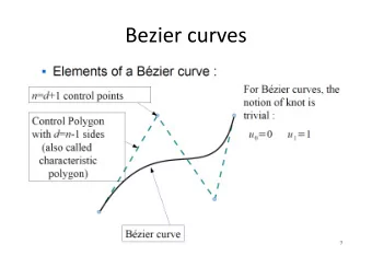
Bézier Curves Properties: • Polynomial curves defined via endpoints and derivative constraints • Derivative constraints defined implicitly through extra control points (that are not interpolated) • They are approximating curves, not interpolating curves

Bézier Curves: Main Idea Polynomial and its derivatives expressed as a cascade of linear interpolations

Bézier Curves: Control Polygon A Bézier curve is completely determined by its control polygon We manipulate the curve by manipulating its polygon

Bézier Curve as a Polynomial

Derivatives of the Bézier Curve

Endpoints and Tangent Constraints General Behaviour • 1 st and 3 rd control points define the endpoints. • 2 nd control point defines the tangent vector at the endpoints.

Generalization to N+1 points Expression in compact form: Curve defined by N linear interpolation cascades (De Casteljau's algorithm): Example for 4 control points and 3 cascades

Bézier and Control Points Expression in compact form:

Bézier Curves: Useful Properties Expression in compact form: 1.Affine Invariance • Transforming a Bézier curve by an affine transform T is equivalent to transforming its control points by T 2.Diminishing Variation • No line will intersect the curve at more points than the control polygon • curve cannot exhibit “excessive fluctuations” 3.Linear Precision • If control poly approximates a line, so will the curve

Bézier Curves: Useful Properties Expression in compact form: 4. Tangents at endpoints are along the 1st and last edges of control polygon:

Bézier Curves: Pros and Cons Advantages: • Intuitive control for N ≤ 3 • Derivatives easy to compute • Nice properties (affine invariance, diminishing variation) Disadvantages: • Scheme is still global (curve is function of all control points)

Reminders

Bezier Basis Matrix A cubic Bezier can be defined with four points where: P 1 ,R 1 at t=0 and P 4 ,R 4 at t=1 for a Hermite. R 1 = 3(P 2 -P 1 ) and R 4 = 3(P 4 -P 3 ). We can thus compute the Bezier Basis Matrix by finding the matrix that transforms [P 1 P 2 P 3 P 4 ] T into [P 1 P 4 R 1 R 4 ] T i.e. B_H =[ 1 0 0 0 ] [ 0 0 0 1] [-3 3 0 0] [ 0 0 -3 3] M bezier =M hermite * B_H

Bezier Basis Functions [ -1 3 -3 1 ] [ 3 -6 3 0 ] [ -3 3 0 0 ] [ 1 0 0 0 ] The columns of the Basis Matrix form Basis Functions such that: p(t)= f 1 (t)P 1 + f 2 (t)P 2 + f 3 (t)P 3 + f 4 (t)P 4. From the matrix: n ) * (1-t) (n-i) * t i f i (t) = ( i These are also called Bernstein polynomials.

Basis Functions Basis functions can be thought of as interpolating functions. Note: actual interpolation of any point only happens if its Basis function is 1 and all others are zero at some t. Often Basis functions for design curves sum to 1 for all t. This gives the curve some nice properties like affine invariance and the convex hull property when the function are additionally non-negative.