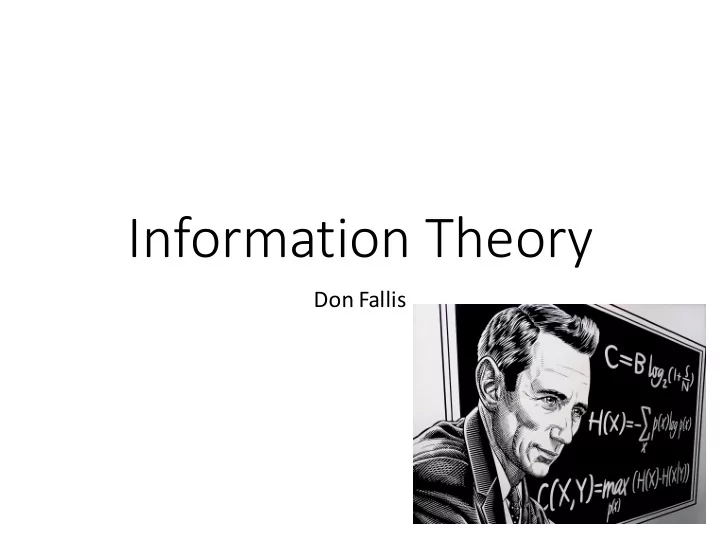
Information Theory Don Fallis Information in the Wild Intentional - PowerPoint PPT Presentation

Information Theory Don Fallis

Information in the Wild

Intentional Information Transfer

Data Storage

Measuring Information

Surprise!

Inversely Related to Probability • The lower the probability of event A, the more information you get by learning A. • The higher the probability of event A, the less information you get by learning A. • So, 1/p(A) is a plausible measure of the information you get by learning A.

Measuring Information 1 2 • S(HEADS) = 1/p(HEADS) = 1/0.5 = 2 1 2 3 4 • S(‘1’) = 1/p(‘1’) = 1/0.25 = 4 1 2 3 4 5 6 7 8 • S(‘2’) = 1/p(‘2’) = 1/0.125 = 8

Measuring Information 1 2 1 1 5 2 2 6 3 3 7 4 4 8 • 2 + 4 ≠ 8 • Log 2 (2) + log 2 (4) = 1 + 2 = 3 = log 2 (8)

Binary Search

Surprise • Surprise of a Fair Coin coming up Heads • S (FC = HEADS) = log 2 ( 1/(1/2) ) = log 2 (2) = 1 bit • Surprise of LLR being at the Left shrub at first time step • S (X 1 = LEFT) = log 2 ( 1/(1/3) ) = log 2 (3) = 1.58 bits • Surprise of a Fire Alarm going off • S (FA = ALARM) = log 2 ( 1/(1/100) ) = log 2 (100) = 6.644 bits

Bits versus Binary Digits

Entropy • Entropy is Average Surprise • Note that this another example of expected value . • Entropy of a Fair Coin • H (FC) = 1/2*log 2 (2) + 1/2*log 2 (2) • H (FC) = 1/2*1 + 1/2*1 = 1 • Entropy of Robot Location at first time step • H (X 1 ) = 1/3*log 2 (3) + 1/3*log 2 (3) + 1/3*log 2 (3) • H (X 1 ) = 1/3*1.58 + 1/3*1.58 + 1/3*1.58 = 1.58 • Entropy of a Fire Alarm • H (FA) = 0.01*log 2 (100) + 0.99*log 2 (1.01) • H (FA) = 0.01*6.644 + 0.99*0.014 = 0.081

Uniform Maximizes Entropy

Amount of Information Transmitted

Noise

Information Channel

Binary Symmetric Channel

Probabilistic Graphical Model • 𝑞 𝑠 | 𝑡 • 𝑞 𝑡 𝛀 SR 𝚾 S R 0 R 1 S 0 q S 0 1-p p S 1 1-q S 1 p 1-p

Mutual Information

Worst-Case Scenario (Independent)

Best-Case Scenario (Perfectly Correlated) • 𝐼 𝑌 = 𝐼 𝑍 = 𝑁𝐽 𝑌 & 𝑍

Everything In Between • 𝑁𝐽 𝑌 & 𝑍 = 𝐼 𝑌 + 𝐼 𝑍 − 𝐼(𝑌 & 𝑍)

Measuring Mutual Information • Mutual Information is Expected Reduction in Uncertainty • Note that this another example of expected value . • Suppose that you see a Yellow flash … • Your credences shift from (1/3, 1/3, 1/3) to (1/2, 1/2, 0) • The entropy of your credences shifts from 1.58 to 1 • So, there is a reduction in entropy of 0.58 • Suppose that you see a White flash … • Your credences shift from (1/3, 1/3, 1/3) to (0, 0, 1) • The entropy of your credences shifts from 1.58 to 0 • So, there is a reduction in entropy of 1.58 • Take a Weighted Average … • The probability of a Yellow flash is 2/3 • The probability of a White flash is 1/3 • So, the expected reduction in entropy is 2/3*0.58 + 1/3*1.58 = 0.92

Firefly Entropy • H (H) = 1/3*log 2 (3) + 1/3*log 2 (3) + 1/3*log 2 (3) • H (H) = 1/3*1.58 + 1/3*1.58 + 1/3*1.58 = 1.58 • H (E) = 2/3*log 2 (1.5) + 1/3*log 2 (3) • H (E) = 2/3*0.58 + 1/3*1.58 = 0.92 • 𝑞 ℎ & 𝑓 , 𝑞 ℎ , and 𝑞(𝑓) H↓ E→ YELLOW WHITE total H GOOD 1/3 0 1/3 BAD 1/3 0 1/3 UGLY 0 1/3 1/3 total E 2/3 1/3

More Firefly Entropy • H (H&E) = 1/3*log 2 (3) + 0*log 2 (0) + 1/3*log 2 (3) + 0*log 2 (0) + 0*log 2 (0) + 1/3*log 2 (3) • H (H&E) = 1/3*1.58 + 0*(-∞) + 1/3*1.58 + 0*(-∞) + 0*(-∞) + 1/3*1.58 = 1.58 • 𝑞 ℎ & 𝑓 , 𝑞 ℎ , and 𝑞(𝑓) H↓ E→ YELLOW WHITE total H GOOD 1/3 0 1/3 BAD 1/3 0 1/3 UGLY 0 1/3 1/3 total E 2/3 1/3

Firefly Mutual Information • MI (H&E) = H (H) + H (E) – H (H&E) • MI (H&E) = 1.58 + 0.92 – 1.58 = 0.92 • 𝑞 ℎ & 𝑓 , 𝑞 ℎ , and 𝑞(𝑓) H↓ E→ YELLOW WHITE total H GOOD 1/3 0 1/3 BAD 1/3 0 1/3 UGLY 0 1/3 1/3 total E 2/3 1/3

Robot Localization #1 • H (X 1 ) = 1/3*log 2 (3) + 1/3*log 2 (3) + 1/3*log 2 (3) • H (X 1 ) = 1/3*1.58 + 1/3*1.58 + 1/3*1.58 = 1.58 • H (X 2 ) = 1/12*log 2 (12) + 1/3*log 2 (3) + 7/12*log 2 (1.71) • H (X 2 ) = 1/12*3.58 + 1/3*1.58 + 7/12*0.78 = 1.28 • 𝑞 𝑦 1 & 𝑦 2 , 𝑞 𝑦 1 , and 𝑞 𝑦 2 X 1 ↓ X 2 → left middle right total X 1 left 1/12 1/4 0 1/3 middle 0 1/12 1/4 1/3 right 0 0 1/3 1/3 total X 2 1/12 1/3 7/12

Robot Localization #1 • H (X 1 &X 2 ) = 1/12*log 2 (12) + 1/4*log 2 (4) + 1/12*log 2 (12) + 1/4*log 2 (4) + 1/3*log 2 (3) • H (X 1 &X 2 ) = 1/12*3.58 + 1/4*2 + 1/12*3.58 + 1/4*2 + 1/3*1.58 = 2.13 • 𝑞 𝑦 1 & 𝑦 2 , 𝑞 𝑦 1 , and 𝑞 𝑦 2 X 1 ↓ X 2 → left middle right total X 1 left 1/12 1/4 0 1/3 middle 0 1/12 1/4 1/3 right 0 0 1/3 1/3 total X 2 1/12 1/3 7/12

Robot Localization #1 • MI (X 1 &X 2 ) = H (X 1 ) + H (X 2 ) – H (X 1 &X 2 ) • MI (X 1 &X 2 ) = 1.58 + 1.28 – 2.13 = 0.74 • 𝑞 𝑦 1 & 𝑦 2 , 𝑞 𝑦 1 , and 𝑞 𝑦 2 X 1 ↓ X 2 → left middle right total X 1 left 1/12 1/4 0 1/3 middle 0 1/12 1/4 1/3 right 0 0 1/3 1/3 total X 2 1/12 1/3 7/12

Robot Localization #1 • H (X 1 ) = 1/3*log 2 (3) + 1/3*log 2 (3) + 1/3*log 2 (3) • H (X 1 ) = 1/3*1.58 + 1/3*1.58 + 1/3*1.58 = 1.58 • H (O 1 ) = 2/3*log 2 (1.5) + 1/3*log 2 (3) • H (O 1 ) = 2/3*0.58 + 1/3*1.58 = 0.92 • 𝑞 𝑦 1 & 𝑝 1 , 𝑞 𝑦 1 , and 𝑞 𝑝 1 X 1 ↓ O 1 → hot cold total X 1 left 1/3 0 1/3 middle 0 1/3 1/3 right 1/3 0 1/3 total O 1 2/3 1/3

Robot Localization #1 • H (X 1 &O 1 ) = 1/3*log 2 (3) + 0*log 2 (0) + 0*log 2 (0) + 1/3*log 2 (3) + 1/3*log 2 (3) + 0*log 2 (0) • H (X 1 &O 1 ) = 1/3*1.58 + 0*(-∞) + 0*(-∞) + 1/3*1.58 + 1/3*1.58 + 0*(-∞) = 1.58 • 𝑞 𝑦 1 & 𝑝 1 , 𝑞 𝑦 1 , and 𝑞 𝑝 1 X 1 ↓ O 1 → hot cold total X 1 left 1/3 0 1/3 middle 0 1/3 1/3 right 1/3 0 1/3 total O 1 2/3 1/3

Robot Localization #1 • MI (X 1 &O 1 ) = H (X 1 ) + H (O 1 ) – H (X 1 &O 1 ) • MI (X 1 &O 1 ) = 1.58 + 0.92 – 1.58 = 0.92 • 𝑞 𝑦 1 & 𝑝 1 , 𝑞 𝑦 1 , and 𝑞 𝑝 1 X 1 ↓ O 1 → hot cold total X 1 left 1/3 0 1/3 middle 0 1/3 1/3 right 1/3 0 1/3 total O 1 2/3 1/3