Inference in hybrid Bayesian networks with H. Langseth, T.D. - PowerPoint PPT Presentation
Inference with MoTBFs Inference in hybrid Bayesian networks with H. Langseth, T.D. Nielsen, R. Rum , mixtures of truncated basis functions A. Salmer on MoTBFs Operations Helge Langseth (1) , Thomas D. Nielsen (2) , Rafael Rum
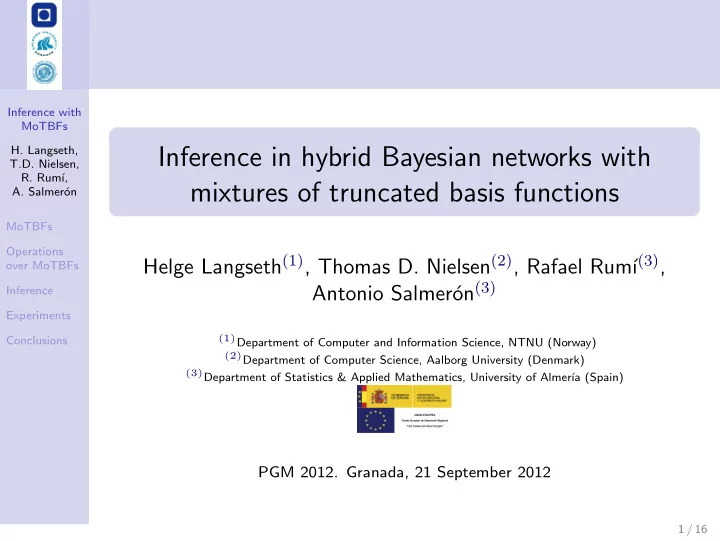
Inference with MoTBFs Inference in hybrid Bayesian networks with H. Langseth, T.D. Nielsen, R. Rum´ ı, mixtures of truncated basis functions A. Salmer´ on MoTBFs Operations Helge Langseth (1) , Thomas D. Nielsen (2) , Rafael Rum´ ı (3) , over MoTBFs on (3) Inference Antonio Salmer´ Experiments (1) Department of Computer and Information Science, NTNU (Norway) Conclusions (2) Department of Computer Science, Aalborg University (Denmark) (3) Department of Statistics & Applied Mathematics, University of Almer´ ıa (Spain) PGM 2012. Granada, 21 September 2012 1 / 16
Introduction Inference with MoTBFs H. Langseth, T.D. Nielsen, R. Rum´ ı, A. Salmer´ on MoTBFs MoTBFs provide a flexible framework for hybrid BNs. Operations Accurate approximation of known models. over MoTBFs Inference Learning from data. Experiments Inference? Conclusions 2 / 16
Mixtures of truncated basis functions (MoTBFs) Inference with MoTBFs H. Langseth, T.D. Nielsen, R. Rum´ ı, A. Salmer´ on In what concerns inference in Bayesian networks, initially MoTBFs we only have two types of MoTBFs: univariate and Operations over MoTBFs conditional. Inference Any other potential showing up during inference is the Experiments result of operating over them, namely applying Conclusions marginalisation and combination. 3 / 16
Mixtures of truncated basis functions (MoTBFs) Inference with Definition (Univariate MoTBF density) MoTBFs H. Langseth, An unconditional MoTBF density over X is: T.D. Nielsen, R. Rum´ ı, A. Salmer´ on m − 1 MoTBFs � f ( x ) = a i ψ i ( x ) x ∈ Ω X , Operations i =0 over MoTBFs Inference where Experiments ψ = { ψ 0 ( x ) , . . . , ψ m − 1 ( x ) } Conclusions is the set of basis functions for X . Particular cases MTEs: Ψ = { 1 , exp( − x ) , exp( x ) , exp( − 2 x ) , exp(2 x ) , . . . } . MOPs: Ψ = { x i , i = 0 , 1 , . . . } . 4 / 16
Mixtures of truncated basis functions (MoTBFs) Inference with Definition (Univariate MoTBF density) MoTBFs H. Langseth, An unconditional MoTBF density over X is: T.D. Nielsen, R. Rum´ ı, A. Salmer´ on m − 1 MoTBFs � f ( x ) = a i ψ i ( x ) x ∈ Ω X , Operations i =0 over MoTBFs Inference where Experiments ψ = { ψ 0 ( x ) , . . . , ψ m − 1 ( x ) } Conclusions is the set of basis functions for X . Particular cases MTEs: Ψ = { 1 , exp( − x ) , exp( x ) , exp( − 2 x ) , exp(2 x ) , . . . } . MOPs: Ψ = { x i , i = 0 , 1 , . . . } . 4 / 16
Mixtures of truncated basis functions (MoTBFs) Inference with MoTBFs H. Langseth, T.D. Nielsen, Definition (Conditional MoTBF density) R. Rum´ ı, A. Salmer´ on Y and Z : discrete and continuous variables. MoTBFs Domain of Z divided into k hypercubes. Operations over MoTBFs For each y , and each hypercube j = 1 , . . . , k , the Inference conditional MoTBF density of X given Z and Y is Experiments Conclusions m − 1 � f ( x | z , y ) = a i,j ψ i ( x ) i =0 5 / 16
Mixtures of truncated basis functions (MoTBFs) Inference with Potential advantages of MoTBFs for inference MoTBFs H. Langseth, Univariate MoTBFs do not require domain splitting (unlike T.D. Nielsen, R. Rum´ ı, classical approach to MTEs and MOPs). A. Salmer´ on Conditional MoTBFs are piecewise univariate over the MoTBFs head variable. Operations over MoTBFs As a consequence, each variable in the BN explicitly Inference appears in only one potential initially. Experiments If a variable appears in a potential not as a head variable, Conclusions it only determines the hypercubes of the conditional density. One can consider a fixed set of possible split points for each variable, regardless of the function where it appears. There is no need to explicitly store the basis functions. 6 / 16
Combination Inference with MoTBFs m − 1 m − 1 H. Langseth, � a 1 � a 2 T.D. Nielsen, f ( x 1 ) = i,h ψ i ( x 1 ) ; f ( x 2 ) = i,t ψ i ( x 2 ) R. Rum´ ı, A. Salmer´ on i =0 i =0 MoTBFs Operations over MoTBFs Inference Experiments �� m − 1 � �� m − 1 � Conclusions i =0 a 1 i =0 a 2 f ( x 1 , x 2 ) = i,h ψ i ( x 1 ) i,t ψ i ( x 2 ) 7 / 16
Combination Inference with MoTBFs m − 1 m − 1 H. Langseth, � a 1 � a 2 T.D. Nielsen, f ( x 1 ) = i,h ψ i ( x 1 ) ; f ( x 2 ) = i,t ψ i ( x 2 ) R. Rum´ ı, A. Salmer´ on i =0 i =0 MoTBFs Operations over MoTBFs Inference Experiments �� m − 1 � �� m − 1 � Conclusions i =0 a 1 i =0 a 2 f ( x 1 , x 2 ) = i,h ψ i ( x 1 ) i,t ψ i ( x 2 ) MoTBF potential 7 / 16
Combination Inference with MoTBFs m − 1 m − 1 H. Langseth, � a 1 � a 2 T.D. Nielsen, f ( x 1 ) = i,h ψ i ( x 1 ) ; f ( x 2 ) = i,t ψ i ( x 2 ) R. Rum´ ı, A. Salmer´ on i =0 i =0 MoTBFs Operations over MoTBFs Inference Experiments �� m − 1 � �� m − 1 � Conclusions i =0 a 1 i =0 a 2 f ( x 1 , x 2 ) = i,h ψ i ( x 1 ) i,t ψ i ( x 2 ) MoTBF potential MoTBF potential 7 / 16
Combination Inference with MoTBFs m − 1 m − 1 H. Langseth, � a 1 � a 2 T.D. Nielsen, f ( x 1 ) = i,h ψ i ( x 1 ) ; f ( x 2 ) = i,t ψ i ( x 2 ) R. Rum´ ı, A. Salmer´ on i =0 i =0 MoTBFs Factorised MoTBF potential Operations over MoTBFs Inference Experiments �� m − 1 � �� m − 1 � Conclusions i =0 a 1 i =0 a 2 f ( x 1 , x 2 ) = i,h ψ i ( x 1 ) i,t ψ i ( x 2 ) MoTBF potential MoTBF potential 7 / 16
Marginalisation Inference with MoTBFs Proposition H. Langseth, T.D. Nielsen, R. Rum´ ı, A. Salmer´ on f Z \{ Z j } ( z 1 , . . . , z j − 1 , z j +1 , . . . , z c ) = MoTBFs r m − 1 m − 1 Operations � � � � � a j over MoTBFs a i . s, · , ( h,l ) ψ s ( z i ) ψ s ( z j ) dz j s, · , ( h,l ) Inference Ω l s =0 s =0 l =1 i � = j Zj Experiments Conclusions Bad news: NOT a factorised MoTBF potential! Good news: the integrals can be computed off-line, prior to inference, if the split points are fixed. 8 / 16
Marginalisation Inference with MoTBFs Proposition H. Langseth, T.D. Nielsen, R. Rum´ ı, A. Salmer´ on f Z \{ Z j } ( z 1 , . . . , z j − 1 , z j +1 , . . . , z c ) = MoTBFs r m − 1 m − 1 Operations � � � � � a j over MoTBFs a i . s, · , ( h,l ) ψ s ( z i ) ψ s ( z j ) dz j s, · , ( h,l ) Inference Ω l s =0 s =0 l =1 i � = j Zj Experiments Conclusions Bad news: NOT a factorised MoTBF potential! Good news: the integrals can be computed off-line, prior to inference, if the split points are fixed. This kind of potential is called SP factorised MoTBF potential 8 / 16
Combination of SP factorised potentials Inference with MoTBFs H. Langseth, T.D. Nielsen, r 1 r 2 R. Rum´ ı, � � f l f m A. Salmer´ on f X 1 ( x 1 ) = X 1 ( x 1 ) ; f X 2 ( x 2 ) = X 2 ( x 2 ) l =1 m =1 MoTBFs Operations The combination of f X 1 and f X 2 is a new potential over over MoTBFs Inference variables X 12 = X 1 ∪ X 2 defined as Experiments r 1 r 2 Conclusions X 1 ( x ↓ X 1 X 2 ( x ↓ X 2 � � f l 12 ) f m f ( x 12 ) = 12 ) , l =1 m =1 which is an SP factorised potential. 9 / 16
Marginalisation of SP factorised potentials Inference with MoTBFs H. Langseth, r T.D. Nielsen, � R. Rum´ ı, f l f Z ( z ) = Z ( z ) A. Salmer´ on l =1 MoTBFs Operations over MoTBFs Inference f Z \{ Z j } ( z 1 , . . . , z j − 1 , z j +1 , . . . , z c ) = Experiments r Conclusions � f l Z \{ Z j } ( z 1 , . . . , z j − 1 , z j +1 , . . . , z n ) l =1 Again, it is an SP factorised potential. 10 / 16
Marginalisation of SP factorised potentials Inference with MoTBFs H. Langseth, r T.D. Nielsen, � R. Rum´ ı, f l f Z ( z ) = Z ( z ) A. Salmer´ on l =1 MoTBFs Operations over MoTBFs Inference f Z \{ Z j } ( z 1 , . . . , z j − 1 , z j +1 , . . . , z c ) = Experiments r Conclusions � f l Z \{ Z j } ( z 1 , . . . , z j − 1 , z j +1 , . . . , z n ) l =1 Again, it is an SP factorised potential. 10 / 16
Why are SP factorised potentials of interest? Inference with MoTBFs H. Langseth, T.D. Nielsen, R. Rum´ ı, A. Salmer´ on They are closed for marginalisation and combination. MoTBFs Hence, inference algorithms as Shenoy-Shafer and Variable Operations over MoTBFs Elimination can be used. Inference Operations over them are lazy by nature, i.e., handling Experiments them actually consists of handling sets of function Conclusions (storing, indexing and retrieving them). 11 / 16
Classical MTE calculations vs. MoTBFs Inference with MoTBFs H. Langseth, T.D. Nielsen, R. Rum´ ı, Two experiments conducted A. Salmer´ on 1 MoTBF vs. classical MTE approach: MoTBFs No splits in head variables. Operations Fixed splits in conditionals. over MoTBFs Inference 2 Lazy operations on SP factorised potentials vs. classical Experiments MTE operations. Conclusions Random split points everywhere. We use the Variable Elimination algorithm. 12 / 16
Classical MTE calculations vs. MoTBFs Inference with MoTBFs H. Langseth, T.D. Nielsen, R. Rum´ ı, Two experiments conducted A. Salmer´ on 1 MoTBF vs. classical MTE approach: MoTBFs No splits in head variables. Operations Fixed splits in conditionals. over MoTBFs Inference 2 Lazy operations on SP factorised potentials vs. classical Experiments MTE operations. Conclusions Random split points everywhere. We use the Variable Elimination algorithm. 12 / 16
Recommend
More recommend
Explore More Topics
Stay informed with curated content and fresh updates.
