INF5110 Compiler Construction Code generation Spring 2016 1 / 123 - PowerPoint PPT Presentation
INF5110 Compiler Construction Code generation Spring 2016 1 / 123 Outline 1. Code generation Intro 2AC and costs of instructions Basic blocks and control-flow graphs Code generation algo Global analysis Bibs 2 / 123 Outline 1. Code
Data flow analysis in general • general analysis technique working on CFGs • many concrete forms of analyses • such analyses: basis for (many) optimizations • data : info stored in memory/temporaries/registers etc. • control : • movement of the instruction pointer • abstractly represented by the CFG • inside elementary blocks: increment of the IS • edges of the CFG: (conditional) jumps • jumps together with RTE and calling convention Data flowing from (a) to (b) Given the control flow (normally as CFG): is it possible (or is it guaranteed) that some “data” originating at one control-flow point (a) reach another control flow point (b). 26 / 123
Data flow as abstraction • data flow analysis: fundamental and important static analysis technique • it’s impossible to decide statically if data from (a) actually “flows to” (b) ⇒ approximative • therefore: work on the CFG: if there is two options/outgoing edges: consider both • Data-flow answers therefore approximatively • if it’s possible that the data flows from (a) to (b) • it’s neccessary or unavoidable that data flows from (a) to (b) • for basic blocks : exact answers possible 4 4 static simulation here was done for basic blocks only and for the purpose of translation . The translation of course needs to be exact, non-approximative. Symbolic evaluation also exist (also for other purposes) in more general forms, especially also working approximatively on abstractions. 27 / 123
Data flow analysis: Liveness • prototypical / important data flow analysis • especially important for register allocation Basic question When (at which control-flow point) can I be sure that I don’t need a specific variable (temporary, register) any more? • optimization: if sure that not needed in the future: register can be used otherwise Definition (Live) a variable is live at a given control-flow point if there exists an execution starting from there, where the variable is used in the future. a a That corresponds to static liveness (the notion the static liveness analysis deals with. A variable in a given concrete execution of a program is dynamically live if in the future, it is still needed (or, for non-deterministic programs: if there exists a future, where it’s still used. Dynamic liveness is undecidable, obviously. 28 / 123
Definitions and uses of variables • when talking about “varaibles”: also temporary variables are meant. • basic notions underlying most data-flow analyses (including liveness analysis) • here: def’s and uses of variables (or temporaries etc) • all data, including intermediate results) has to be stored somewhere, in variables, temporaries, etc. • a “definition” of x = assignment to x (store to x ) • a “use” of x : read content of x (load x ) • variables can occur more than once, so • a definition/use refers to instances or occurrences of variables (“use of x in line l ” or “use of x in block b ”) • same for liveness: “ x is live here, but not there” 29 / 123
Defs, uses, and liveness • x is “defined” (= assigned 0: x = v + w to) in 0 and 4 • x is live “in” (= at the end of) block 2, as it may be . . . used in 5 • a non-live variable at some point: “dead” which means: 2: a = x + c the corresponding memory can be reclaimed. 4: x = w 3: x =u + v • note : here liveness across block-boundaries = “global” (but blocks contain only one 5: d = x + y instruction here) 30 / 123
Def-use or use-def analysis • use-def: given a “use”: determine all possible “definitions” 5 • def-use: given a “def”: determine all possible “uses” • for straight-line-code/inside one basic block • deterministic: each line has has exactly one place where a given variable has been assigned to last (or else not assigned to in the block). Equivalently for uses. • for whole CFG: • approximative (“may be used in the future”) • more advanced techiques (caused by presence of loops/cycles) • def-use analysis: • closely connected to liveness analysis (basically the same) • prototypical data-flow question (same for use-def analysis), related to many data-flow analyses (but not all) • Side remark: Static single-assignment (SSA) format: • at most one assignment per variable. • “definition” (place of assignment) for each variable thus clear from its name 5 remember: “defs” and “uses” refer to instances of definitions/assignments in the graph 31 / 123
Calculation of def/uses (or liveness . . . ) • three levels of complication 1. inside basic block 2. branching (but no loops) 3. Loops 4. [even more complex: inter-procedural analysis] For SLC/inside basic block For whole CFG • determnistic result • iterative algo needed • simple “one-pass” treatment • dealing with enough non-determinism: over-approximation • similar to “static simulation” • “closure” algorithms, similar to the way e.g., dealing with first and follow sets • = fix-point algorithms 32 / 123
Inside one block: optimizing use of temporaries • simple setting: intra -block analysis & optimization, only • temporaries: • symbolic representations to hold intermediate results • generated on request, assuming unbounded numbers • intentions: use registers • limited about of register available (platform dependent) Assumption • temp’s don’t transfer data accross blocks ( / = program var’s) ⇒ temp’s dead at the beginning and at the end of a block • but: variables have to be considered live at the end of a block (block-local analysis, only) 33 / 123
Intra-block liveness • neither temp’s nor vars: “single assignment”, • but first occurrence of a temp in a block: a definition (but for temps it t1 := a − b would often be the case) t2 := t1 ∗ a a := t1 ∗ t2 • let’s call operand: variables or temp’s t1 := t1 − c a := t1 ∗ a • next use of an operand: • uses of operands: on the lhs’s, definitions on the rhs’s • not good enough to say “ t 1 is live in line 4” Note: the TAIC may allow also literal constants as operator arguments, they don’t play a role right now. 34 / 123
DAG of the block ∗ a • no linear order (as in code), only partial order • the next use: meaningless ∗ a − t 1 • but: all “next” uses visible (if any) ∗ • node = occurrences of a t 2 variable on the rhs (“definitions”) − t 1 • e.g.: the “lower node” for “defining” assigning to t 1 has /three uses a 0 c 0 b 0 35 / 123
DAG / SA ∗ a 2 t 1 ∗ a 1 − 1 t 0 ∗ 2 t 0 − 1 a 0 c 0 b 0 36 / 123
Intra-block liveness: idea of algo • liveness-status of an operand: different from lhs vs. rhs in a given instruction a • informal definition: an operand is live at some occurrence, if it’s used some place in the future a but if one occurrence of (say) x in a rhs x + x is live, so is the other occurrence. Definition (consider statement x 1 ∶= x 2 op x 3 ) • A variable x is live at the beginning of x 1 ∶= x 2 op x 3 , if 1. if x is the same variable than x 2 or x 3 , or 2. if x live at its end , provided x and x 1 are different variables • A variable x is live at the end of an instruction, • if it’s live at beginning of the next instruction • if no next instruction • temp’s are dead • user-leval variables are (assumed) live 37 / 123
Liveness Previous “inductive” definition expresses liveness status of variables before a statement dependent on the liveness status of variables after a statement (and the variables used in the statement) • core of a straightforward iterative algo • simple backward scan 6 • the algo we sketch: • not just boolean info (live = yes/no), instead: • operand live? • yes, and with next use inside is block (and indicate instruction where) • yes, but with no use inside this block • not live: • even more info: not just that but indicate, where’s the next use 6 Remember: intra-block/SLC. In the presence of loops/analysing a complete CFG, a simple 1-pass does not suffice. More advanced techniques (“multiple-scans” = fixpoint calculations) are needed then. 38 / 123
Algo: dead or alive (binary info only) // −−−−− i n i t i a l i s e T −−−−−−−−−−−−−−−−−−−−−−−−−−−− e n t r i e s : T[ i , x ] := D f o r a l l except : f o r a l l v a r i a b l e s a // but not temps T[ n , a ] := L , // −−−−−−− backward pass −−−−−−−−−−−−−−−−−−−−−−−−−−−− f o r i n s t r u c t i o n i = n − 1 down to 0 l e t c u r r e n t i n s t r u c t i o n i : x ∶= y op z ; T[ i . y ] := L T[ i . z ] := L T[ i . x ] := D // note o r d e r ; x can ‘ ‘ equal ’ ’ y or z end • Data structure T : table, mapping for each line/instruction i and variable: boolean status of “live”/“dead” • represents liveness status per variable at the end (i.e. rhs) of that line • basic block: n instructions, from 1 until n , where “line 0” represents the sentry imaginary line “before” the first line (no instruction in line 0) • backward scan through instructions/lines from n to 0 39 / 123
Algo ′ : dead or else: alive with next use • More refined information • not just binary “dead-or-alive” but next-use info ⇒ three kinds of information 1. Dead: D 2. Live: • with local line number of next use : L ( n ) • potential use of outside local basic block L (�) • otherwise: basically the same algo // −−−−− i n i t i a l i s e T −−−−−−−−−−−−−−−−−−−−−−−−−−−− f o r a l l e n t r i e s : T[ i , x ] := D except : v a r i a b l e s a // but temps f o r a l l not T[ n , a ] := L (�) , // −−−−−−− backward pass −−−−−−−−−−−−−−−−−−−−−−−−−−−− f o r i n s t r u c t i o n i = n − 1 down to 0 l e t c u r r e n t i n s t r u c t i o n i : x ∶= y op z ; T[ i , y ] := L ( i + 1 ) T[ i , z ] := L ( i + 1 ) T[ i , x ] := D // note o r d e r ; x can ‘ ‘ equal ’ ’ y or z end 40 / 123
Run of the algo ′ line a b c t 1 t 2 [ 0 ] L ( 1 ) L ( 1 ) L ( 4 ) L ( 2 ) D L ( 2 ) L ( � ) L ( 4 ) L ( 2 ) 1 D 2 L ( � ) L ( 4 ) L ( 3 ) L ( 3 ) D 3 L ( 5 ) L ( � ) L ( 4 ) L ( 4 ) D 4 L ( 5 ) L ( � ) L ( � ) L ( 5 ) D 5 L ( � ) L ( � ) L ( � ) D D t1 := a − b t2 := t1 ∗ a a := t1 ∗ t2 t1 := t1 − c a := t1 ∗ a 41 / 123
Liveness algo remarks • here: T data structure traces (L/D) status per variable × “line” • in the remarks in the notat: • alternatively: store liveness-status per variable only • works as well for one-pass analyses (but only without loops) • this version here: corresponds better to global analysis: 1 line can be seen as one small basic block 42 / 123
Outline 1. Code generation Intro 2AC and costs of instructions Basic blocks and control-flow graphs Code generation algo Global analysis Bibs 43 / 123
Simple code generation algo • simple algo: intra-block code generation • core problem: register use • register allocation & assignment 7 • hold calculated values in registers longest possibe • intra-block only ⇒ at exit: • all variables stored back to main memory • all temps assumed “lost” • remember: assumptions in the intra-block liveness analysis 7 some distinguish register allocation: “should the data be held in register (and how long)” vs. register assignment: “which of available register to use for that” 44 / 123
Limitations of the code generation • local intra block: • no analysis across blocks • no procedure calls etc • no complex data structures • arrays • pointers • . . . some limitations on how the algo itself works for one block • read-only variables: never put in registers, even if variable is repeatedly read • algo works only with the temps/variables given and does not come up with new ones • for instance: DAGs could help • no semantics considered • like commutativity : a + b equals b + a 45 / 123
Purpose and “signature” of the getreg function • one core of the code generation algo • simple code-generation here ⇒ simple getreg getreg function available: liveness/next-use info Input: TAIC-instruction x ∶= y op z Output: return location where x is to be stored • location: register (if possible) or memory location 46 / 123
Coge generation invariant it should go without saying . . . : Basic safetey invariant At each point, “live” variables (with or without next use in the current block) must exist in at least one location • another (specific) invariant: the location returned by getreg: the one where the rhs of a 3AIC assignment ends up 47 / 123
Register and address-descriptors • code generation/ getreg : keep track of 1. register contents 2. addresses for names Address descriptor • tracking location(s) where Register descriptor current value of name can • tracking current content of be found reg’s (if any) • possible locations: register, • consulted when new reg stack location, main memory needed • > 1 location possible (but • as said: at block entry, not due to assume all regs unused overapproximation, exact tracking) 48 / 123
Code generation algo for x ∶= y op z 1. determine location (preferably register) for result L = g e t r e g ( ‘ ‘ x := y op z ’ ’ ) 2. make sure, that the value of y is in L : • consult address descriptor for y ⇒ current locations y ′ for y • choose the best location y ′ from those (register) • if value of y not in L, generate M O V y ’ , L 3. generate OP z ’ , L // z ’ : a c u r r e n t l o c a t i o n of z ( p r e f e r reg ’ s ) • update address descriptor x ↦ L • if L is a reg: update reg descriptor L ↦ x 4. exploit liveness/next use info: update register descriptors 49 / 123
Skeleton code generation algo for x ∶= y op z l = getreg ( ‘ ‘ x:= y op z ’ ’ ) // t a r g e t l o c a t i o n f o r x i f l ∉ T a ( y ) then l e t l y ∈ T a ( y ) ) in emit ("MOV l y , l " ) ; z ′ ∈ T a ( z ) ) l e t in emit ("OP z ′ , l " ) ; • “skeleton” • non-deterministic: we igored how to choose z ′ and y ′ • we ignore book-keeping in the name and address descriptor tables • details of getreg hidden. 50 / 123
Non-deterministic code generation algo for x ∶= y op z L = getreg ( ‘ ‘ x:= y op z ’ ’ ) // gener ate t a r g e t l o c a t i o n f o r x i f L ∉ T a ( y ) y ′ ∈ T a ( y ) ) // p i c k a l o c a t i o n y then l e t f o r in emit (MOV y ’ , L) skip ; e l s e z ′ ∈ T a ( z ) ) ( ‘ ‘OP z ′ , L ’ ’ ) ; l e t in emit T a ∶= T a [ x ↦ L ] ; i f L i s a r e g i s t e r then T r ∶= T r [ L ↦ x ] 51 / 123
Code generation algo for x ∶= y op z l = getreg (" i : x := y op z ") // i i n s t r u c t i o n s l i n e number/ l a b f o r i f l ∉ T a ( y ) then l e t l y = best ( T a ( y ) ) in emit (" MOV l y , l ") e l s e skip ; l e t l z = best ( T a ( z ) ) in emit (" OP l z , l " ) ; T a ∶ = T a /( _ ↦ l ) ; T a ∶ = T a [ x ↦ l ] ; T r ∶ = T r [ l ↦ x ] ; i f ¬ T live [ i , y ] and T a ( y ) = r then T r ∶ = T r /( r ↦ y ) i f ¬ T live [ i , z ] and T a ( z ) = r then T r ∶ = T r /( r ↦ z ) 52 / 123
Code generation algo for x ∶= y op z (Notat) l = getreg (" x := y op z ") i f l ∉ T a ( y ) then l e t l y = best ( T a ( y ) ) in emit (" MOV l y , l ") e l s e skip ; l e t l z = best ( T a ( z ) ) in emit (" OP l z , l " ) ; T a ∶ = T a /( _ ↦ l ) ; T a ∶ = T a [ x ↦ l ] ; T r ∶ = T r [ l ↦ x ] 53 / 123
Exploit liveness/next use info: recycling registers • register descriptors: don’t update themselves during code generation • once set (for instance as R 0 ↦ t ), the info stays, unless reset • thus in step 4 for z ∶= x op y : to exploit liveness info by recycling reg’s if y and/or z are currently • not live and are • in registers , ⇒ “wipe” the corresponding info from the corresponding register descriptors • side remark: for address descriptor • no such “wipe” neeed, because it won’t make a difference ( y and/or z are not-live anyhow) • their address descriptor wont’ be consulted further in the block 54 / 123
getreg algo: x ∶= y op z • goal: return a location for x • basically: check possibilities of register uses, • start with the cheapest option do the following steps, in that order 1. in place if x is in a register already (and if that’s fine otherwise), then return the register. 2. new register if there’s an unsused register: return that 3. purge filled register choose more or less cleverly a filled register and save its content, if needed, and return that register 4. use main memory if all else fails 55 / 123
getreg algo: x ∶= y op z in more details 1. if • y in register R • R holds no alternative names • y is not live and has no next use after the 3AIC instruction • ⇒ return R 2. else: if there is an empty register R ′ : return R ′ 3. else: if • x has a next use [or operator requires a register] ⇒ • find an occupied register R • store R into M if needed ( MOV R, M )) • don’t forget to update M ’s address descriptor, if needed • return R 4. else: x not used in the block or no suituable occupied register can be found • return x as location L • choice of purged register: heuristics • remember (for step 3): registers may contain value for > 1 variable ⇒ multiple MOV ’s 56 / 123
Sample TAIC d := (a-b) + (a-c) + (a-c) t := a − b u := a − c v := t + u d := v + u line a b c d t u v [ 0 ] L ( 1 ) L ( 1 ) L ( 2 ) D D D D 1 L ( 2 ) L (�) L ( 2 ) L ( 3 ) D D D 2 L (�) L (�) L (�) D L ( 3 ) L ( 3 ) D 3 L (�) L (�) L (�) L ( 4 ) L ( 4 ) D D 4 L (�) L (�) L (�) L (�) D D D 57 / 123
Code sequence 3AIC 2AC reg. descr. addr. descriptor R 0 R 1 a b c d t u v [0] � � a b c d t u v 1 t := a − b MOV a, R0 [ a ] [ R 0 ] ✚ SUB b, R0 t ✚ R 0 R 0 2 u := a − c MOV a, R1 ⋅ [ a ] [ R 0 ] ✚ SUB c, R1 u ✚ R 0 R 1 ✚ 3 v := t + u ADD R1, R0 v ⋅ ✚ R 0 R 0 4 d := v + u ADD R1, R0 ✚ d R 0 ✚ R 0 MOV R0, d R i : unused all var’s in “home position” • address descriptors: “home position” not explictly needed. • for instance: variable a always to be found “at a ”, as indicated in line “0”. • in the table: only changes (from top to bottom) indicated • after line 3: • t dead • t resides in R 0 (and nothing else in R 0 ) → reuse R 0 58 / 123
Outline 1. Code generation Intro 2AC and costs of instructions Basic blocks and control-flow graphs Code generation algo Global analysis Bibs 59 / 123
From “local” to “global” data flow analysis • data stored in variables, and “flows from definitions to uses” • liveness analysis • one prototypical (and important) data flow analysis • so far: intra-block = straight-line code • related to • def-use analysis: given a “definition” of a variable at some place, where it is (potentially) used • use-def : (the inverse question, “reaching definitions” • other similar questions: • has a value of an expression been calculated before (“available expressions”) • will an expression be used in all possible branches (“very busy expressions”) 60 / 123
Global data flow analysis • block-local • block-local analysis (here liveness): exact information possible • block-local liveness: 1 backward scan • important use of liveness: register allocation , temporaries typically don’t survive blocks anyway • global: working on the complete CFG 2 complications • branching: non-determinism , unclear which branch is taken • loops in the program (loops/cycles in the graph): a simple one pass through the graph does not cut it any longer • exact answers no longer possible (undecidable) ⇒ work with safe approximations • this is: general characteristic of DFA 61 / 123
Generalizing block-local liveness analysis • assumptions for block-local analysis • all program variables (assumed) live at the end of each basic block • all temps are assumed dead there. 8 • now: we do better, info accross blocks at the end of each block: which variables may be use used in subsequent block(s). • now: re-use of temporaries (and thus corresponding registers) across blocks possible • remember local liveness algo: determined liveness status per var/temp at the end of each “line/instruction” 9 8 While assuming variables live, even if they are not, is safe, the opposite may be unsafe. The code generator therefore must not reuse temporaries across blocks when doing this assumption. 9 For sake of making a parallel one could: consider each line as individual block. 62 / 123
Connecting blocks in the CFG: inLive and outLive • CFG: • pretty conventional graph (nodes and edges, often designated start and end node) 10 • nodes = basic blocks = contain straight-line code (here 3AIC) • being conventional graphs: • conventional representations possible • E.g. nodes with lists/sets/collections of immediate successor nodes plus immediate predecessor nodes • remember: local liveness status • can be different before and after one single instruction • liveness status before expressed as dependent on status after ⇒ backward scan • Now per block: inLive and outLive 10 For some analyses resp. algos: assumed that the only cycles in the graph are loops . However, the techniques presented here work generally. 63 / 123
inLive and outLive • tracing / approximating set of live variables 11 at the beginning and end per basic block • inLive of a block: depends on • outLive of that block and • the SLC inside that block • outLive of a block: depends on inLive of the successor blocks Approximation: To err on the safe side Judging a variable (statically) live: always safe . Judging wrongly a variable dead (which actually will be used): unsafe • goal: smallest (but safe) possible sets for outLive (and inLive ) 11 to stress “approximation”: inLive and outLive contain sets of statically live variables. If those are dynamically live or not is undecidable. 64 / 123
Example: Faculty CFG • inLive and outLive • picture shows arrows as successor nodes • needed predecessor nodes (reverse arrows) node/block predecessors B 1 ∅ { B 1 } B 2 B 3 { B 2 , B 3 } { B 3 } B 4 { B 1 , B 4 } B 5 65 / 123
Block local info for global liveness/data flow analysis • 1 CFG per procedure/function/method • as for SLG: algo works backwards • for each block: underlying block-local liveness analyis 3-values block local status per variable result of block-local live variable analysis 1. locally live on entry: variable used (before overwritten or not) 2. locally dead on entry: variable overwritten (before used or not) 3. status not locally determined: variable neither assigned to nor read locally • for efficiency: precompute this info, before starting the global iteration ⇒ avoid recomputation for blocks in loops • in the smallish examples: we often do it simply on-the-fly (by “looking at” the blocks’ SLC) 66 / 123
Global DFA as iterative “completion algorithm” • different names for general approach • closure algorithm • fixpoint iteration • basically: a big loop with • iterating a step approaching an intended solution by making current approximation of the solution larger • until the solution stabilizes • similar (for example): calculation of first- and follow-sets • often: realized as worklist algo • named after central data-structure containing the “work-still-to-be-done” • here possible: worklist containing nodes untreated wrt. liveness analysis (or DFA in general) 67 / 123
Example a := 5 L1 : x := 8 y := a + x if_true x=0 goto L4 z := a + x // B3 a := y + z i f _ f a l s e a=0 goto L1 a := a + 1 // B2 y := 3 + x L5 a := x + y r e s u l t := a + z return r e s u l t // B6 L4 : a := y + 8 y := 3 goto L5 68 / 123
CFG: initialization B 0 ∅ a:=5 ∅ • inLive and outLive : ∅ initialized to ∅ x:=8 B 1 y:=a+x everywere ∅ • note: start with ∅ ∅ z:=a+x x:=y+8 (most) unsafe B 3 B 4 a:=y+z y:=3 ∅ ∅ estimation ∅ • extra (return) node a:=a+1 B 2 y:=3+z • but: analysis here ∅ local per procedure , ∅ a:=x+y B 5 only result:=a+z ∅ ∅ B 6 return result ∅ 69 / 123
Iterative algo General schema Initialization start with the “minimal” estimation ( ∅ everywhere) Loop pick one node & update (= enlarge) liveness estimation in connection with that node Until finish upon stabilization. no further enlargement • order of treatment of nodes: in princple arbitrary 12 • in tendency: following edges backwards • comparison: for linear graphs (like inside a block): • no repeat-until-stabilize loop needed • 1 simple backward scan enough 12 There may be more efficient and less efficient orders of treatment. 70 / 123
Liveness: run ∅ B 0 a:=5 ∅ ∅ x:=8 B 1 y:=a+x ∅ ∅ ∅ z:=a+x x:=y+8 B 3 B 4 a:=y+z y:=3 ∅ ∅ ∅ a:=a+1 B 2 y:=3+z ∅ ∅ a:=x+y B 5 result:=a+z ∅ ∅ B 6 return result ∅ 71 / 123
Liveness: run ∅ B 0 a:=5 ∅ ∅ x:=8 B 1 y:=a+x ∅ ∅ ∅ z:=a+x x:=y+8 B 3 B 4 a:=y+z y:=3 ∅ ∅ ∅ a:=a+1 B 2 y:=3+z ∅ ∅ a:=x+y B 5 result:=a+z ∅ { r } B 6 return result ∅ 72 / 123
Liveness: run ∅ B 0 a:=5 ∅ ∅ x:=8 B 1 y:=a+x ∅ ∅ ∅ z:=a+x x:=y+8 B 3 B 4 a:=y+z y:=3 ∅ ∅ ∅ a:=a+1 B 2 y:=3+z ∅ ∅ a:=x+y B 5 result:=a+z { r } { r } B 6 return result ∅ 73 / 123
Liveness: run ∅ B 0 a:=5 ∅ ∅ x:=8 B 1 y:=a+x ∅ ∅ ∅ z:=a+x x:=y+8 B 3 B 4 a:=y+z y:=3 ∅ ∅ ∅ a:=a+1 B 2 y:=3+z ∅ { x , y . z } a:=x+y B 5 result:=a+z { r } { r } B 6 return result ∅ 74 / 123
Liveness: run ∅ B 0 a:=5 ∅ ∅ x:=8 B 1 y:=a+x ∅ ∅ ∅ z:=a+x x:=y+8 B 3 B 4 a:=y+z y:=3 ∅ { x , y , z } ∅ a:=a+1 B 2 y:=3+z { x , y , z } { x , y . z } a:=x+y B 5 result:=a+z { r } { r } B 6 return result ∅ 75 / 123
Liveness: run ∅ B 0 a:=5 ∅ ∅ x:=8 B 1 y:=a+x ∅ ∅ { x , y , z } z:=a+x x:=y+8 B 3 B 4 a:=y+z y:=3 ∅ { x , y , z } ∅ a:=a+1 B 2 y:=3+z { x , y , z } { x , y . z } a:=x+y B 5 result:=a+z { r } { r } B 6 return result ∅ 76 / 123
Liveness: run ∅ B 0 a:=5 ∅ ∅ x:=8 B 1 y:=a+x { x , y , z } ∅ { x , y , z } z:=a+x x:=y+8 B 3 B 4 a:=y+z y:=3 ∅ { x , y , z } ∅ a:=a+1 B 2 y:=3+z { x , y , z } { x , y . z } a:=x+y B 5 result:=a+z { r } { r } B 6 return result ∅ 77 / 123
Liveness: run ∅ B 0 a:=5 ∅ ∅ x:=8 B 1 y:=a+x { x , y , z } ∅ { x , y , z } z:=a+x x:=y+8 B 3 B 4 a:=y+z y:=3 ∅ { x , y , z } { a , x , z } a:=a+1 B 2 y:=3+z { x , y , z } { x , y . z } a:=x+y B 5 result:=a+z { r } { r } B 6 return result ∅ 78 / 123
Liveness: run ∅ B 0 a:=5 ∅ ∅ x:=8 B 1 y:=a+x { x , y , z } ∅ { x , y , z } z:=a+x x:=y+8 B 3 B 4 a:=y+z y:=3 { a , z , x } { x , y , z } { a , x , z } a:=a+1 B 2 y:=3+z { x , y , z } { x , y . z } a:=x+y B 5 result:=a+z { r } { r } B 6 return result ∅ 79 / 123
Liveness: run ∅ B 0 a:=5 ∅ ∅ x:=8 B 1 y:=a+x { x , y , z } { a , x , y } { x , y , z } z:=a+x x:=y+8 B 3 B 4 a:=y+z y:=3 { a , z , x } { x , y , z } { a , x , z } a:=a+1 B 2 y:=3+z { x , y , z } { x , y . z } a:=x+y B 5 result:=a+z { r } { r } B 6 return result ∅ 80 / 123
Liveness: run ∅ B 0 a:=5 ∅ ∅ x:=8 B 1 y:=a+x { a , x , y , z } { a , x , y } { x , y , z } z:=a+x x:=y+8 B 3 B 4 a:=y+z y:=3 { a , z , x } { x , y , z } { a , x , z } a:=a+1 B 2 y:=3+z { x , y , z } { x , y . z } a:=x+y B 5 result:=a+z { r } { r } B 6 return result ∅ 81 / 123
Liveness: run ∅ B 0 a:=5 ∅ { a , z } x:=8 B 1 y:=a+x { a , x , y , z } { a , x , y } { x , y , z } z:=a+x x:=y+8 B 3 B 4 a:=y+z y:=3 { a , z , x } { x , y , z } { a , x , z } a:=a+1 B 2 y:=3+z { x , y , z } { x , y . z } a:=x+y B 5 result:=a+z { r } { r } B 6 return result ∅ 82 / 123
Liveness: run ∅ B 0 a:=5 { a , z } { a , z } x:=8 B 1 y:=a+x { a , x , y , z } { a , x , y } { x , y , z } z:=a+x x:=y+8 B 3 B 4 a:=y+z y:=3 { a , z , x } { x , y , z } { a , x , z } a:=a+1 B 2 y:=3+z { x , y , z } { x , y . z } a:=x+y B 5 result:=a+z { r } { r } B 6 return result ∅ 83 / 123
Liveness: run { z } B 0 a:=5 { a , z } { a , z } x:=8 B 1 y:=a+x { a , x , y , z } { a , x , y } { x , y , z } z:=a+x x:=y+8 B 3 B 4 a:=y+z y:=3 { a , z , x } { x , y , z } { a , x , z } a:=a+1 B 2 y:=3+z { x , y , z } { x , y . z } a:=x+y B 5 result:=a+z { r } { r } B 6 return result ∅ 84 / 123
Liveness example: remarks • the shown traversal strategy is (cleverly) backwards • example resp. example run simplistic: • the loop (and the choice of “evaluation” order): “harmless loop” after having updated the outLive info for B 1 following the edge from B 3 to B 1 backwards (propagating flow from B 1 back to B 3 ) does not increase the current solution for B 3 • no need (in this particular order) for continuing the iterative search for stabilization • in other examples: loop iteration cannot be avoided • note also: end result (after stabilization) independent from evaluation order! (only some strategies may stabilize faster. . . ) 85 / 123
Another example ∅ B 0 x:=5 y:=a-1 ∅ ∅ x:=y+8 B 1 y:=a+x ∅ ∅ ∅ x:=y+x B 3 a:=y+z B 4 y:=3 ∅ ∅ ∅ B 2 y:=3+z ∅ ∅ a:=x+y B 5 result:=a+1 ∅ ∅ B 6 return result ∅ 86 / 123
Another example ∅ B 0 x:=5 y:=a-1 ∅ ∅ x:=y+8 B 1 y:=a+x ∅ ∅ ∅ x:=y+x B 3 a:=y+z B 4 y:=3 ∅ ∅ ∅ B 2 y:=3+z ∅ ∅ a:=x+y B 5 result:=a+1 ∅ { r } B 6 return result ∅ 87 / 123
Another example ∅ B 0 x:=5 y:=a-1 ∅ ∅ x:=y+8 B 1 y:=a+x ∅ ∅ ∅ x:=y+x B 3 a:=y+z B 4 y:=3 ∅ ∅ ∅ B 2 y:=3+z ∅ ∅ a:=x+y B 5 result:=a+1 { r } { r } B 6 return result ∅ 88 / 123
Another example ∅ B 0 x:=5 y:=a-1 ∅ ∅ x:=y+8 B 1 y:=a+x ∅ ∅ ∅ x:=y+x B 3 a:=y+z B 4 y:=3 ∅ ∅ ∅ B 2 y:=3+z ∅ { x , y } a:=x+y B 5 result:=a+1 { r } { r } B 6 return result ∅ 89 / 123
Another example ∅ B 0 x:=5 y:=a-1 ∅ ∅ x:=y+8 B 1 y:=a+x ∅ ∅ ∅ x:=y+x B 3 a:=y+z B 4 y:=3 ∅ { x , y } ∅ B 2 y:=3+z { x , y } { x , y } a:=x+y B 5 result:=a+1 { r } { r } B 6 return result ∅ 90 / 123
Another example ∅ B 0 x:=5 y:=a-1 ∅ ∅ x:=y+8 B 1 y:=a+x ∅ { x , y } ∅ x:=y+x B 3 a:=y+z B 4 y:=3 ∅ { x , y } ∅ B 2 y:=3+z { x , y } { x , y } a:=x+y B 5 result:=a+1 { r } { r } B 6 return result ∅ 91 / 123
Another example ∅ B 0 x:=5 y:=a-1 ∅ ∅ x:=y+8 B 1 y:=a+x { x , y } { x , y } ∅ x:=y+x B 3 a:=y+z B 4 y:=3 ∅ { x , y } ∅ B 2 y:=3+z { x , y } { x , y } a:=x+y B 5 result:=a+1 { r } { r } B 6 return result ∅ 92 / 123
Another example ∅ B 0 x:=5 y:=a-1 ∅ { y , a } x:=y+8 B 1 y:=a+x { x , y } { x , y } ∅ x:=y+x B 3 a:=y+z B 4 y:=3 ∅ { x , y } ∅ B 2 y:=3+z { x , y } { x , y } a:=x+y B 5 result:=a+1 { r } { r } B 6 return result ∅ 93 / 123
Another example ∅ B 0 x:=5 y:=a-1 { y , a } { y , a } x:=y+8 B 1 y:=a+x { x , y } { x , y } ∅ x:=y+x B 3 a:=y+z B 4 y:=3 ∅ { x , y } ∅ B 2 y:=3+z { x , y , a } { x , y } a:=x+y B 5 result:=a+1 { r } { r } B 6 return result ∅ 94 / 123
Another example B 0 { a } x:=5 y:=a-1 { y , a } { y , a } x:=y+8 B 1 y:=a+x { x , y } { x , y } ∅ x:=y+x B 3 a:=y+z B 4 y:=3 ∅ { x , y } ∅ B 2 y:=3+z { x , y , a } { x , y } a:=x+y B 5 result:=a+1 { r } { r } B 6 return result ∅ 95 / 123
Another example B 0 { a } x:=5 y:=a-1 { y , a } { y , a } x:=y+8 B 1 y:=a+x { a , x , y } { x , y } ∅ x:=y+x B 3 a:=y+z B 4 y:=3 ∅ { x , y } { x , z , a } B 2 y:=3+z { x , y , a } { x , y } a:=x+y B 5 result:=a+1 { r } { r } B 6 return result ∅ 96 / 123
Another example B 0 { a } x:=5 y:=a-1 { y , a } { y , a } x:=y+8 B 1 y:=a+x { a , x , y } { x , y } ∅ x:=y+x B 3 a:=y+z B 4 y:=3 { x , z , a } { x , y } { x , z , a } B 2 y:=3+z { x , y , a } { x , y } a:=x+y B 5 result:=a+1 { r } { r } B 6 return result ∅ 97 / 123
Another example B 0 { a } x:=5 y:=a-1 { y , a } { y , a } x:=y+8 B 1 y:=a+x { a , x , y } { x , y } { x , y , z } x:=y+x B 3 a:=y+z B 4 y:=3 { x , z , a } { x , y } { x , z , a } B 2 y:=3+z { x , y , a } { x , y } a:=x+y B 5 result:=a+1 { r } { r } B 6 return result ∅ 98 / 123
Another example B 0 { a } x:=5 y:=a-1 { y , a } { y , a } x:=y+8 B 1 y:=a+x { a , x , y , z } { x , y } { x , y , z } x:=y+x B 3 a:=y+z B 4 y:=3 { x , z , a } { x , y } { x , z , a } B 2 y:=3+z { x , y , a } { x , y } a:=x+y B 5 result:=a+1 { r } { r } B 6 return result ∅ 99 / 123
Another example B 0 { a } x:=5 y:=a-1 { y , a } { y , z , a } x:=y+8 B 1 y:=a+x { a , x , y , z } { x , y } { x , y , z } x:=y+x B 3 a:=y+z B 4 y:=3 { x , z , a } { x , y } { x , z , a } B 2 y:=3+z { x , y , a } { x , y } a:=x+y B 5 result:=a+1 { r } { r } B 6 return result ∅ 100 / 123
Recommend
More recommend
Explore More Topics
Stay informed with curated content and fresh updates.
