INF421, Lecture 7 Sorting Leo Liberti LIX, Ecole Polytechnique, - PowerPoint PPT Presentation
INF421, Lecture 7 Sorting Leo Liberti LIX, Ecole Polytechnique, France INF421, Lecture 7 p. 1/42 Course Objective : teach notions AND develop intelligence Evaluation : TP not en salle info, Contrle la fin. Note: max( CC, 3 4 CC +
The complexity of sorting For any tree T , | V ( T ) | = number of nodes of T Tree depth : max. path length root → leaf in tree A binary tree T with depth ≤ k has | V ( T ) | ≤ 2 k ⇒ The sorting tree T ∗ of best algorithm has | V ( T ∗ ) | ≤ 2 B n � ∀ T ∈ T n , each π ∈ S n appears in a leaf node of T INF421, Lecture 7 – p. 10/42
The complexity of sorting For any tree T , | V ( T ) | = number of nodes of T Tree depth : max. path length root → leaf in tree A binary tree T with depth ≤ k has | V ( T ) | ≤ 2 k ⇒ The sorting tree T ∗ of best algorithm has | V ( T ∗ ) | ≤ 2 B n � ∀ T ∈ T n , each π ∈ S n appears in a leaf node of T ⇒ Any T ∈ T n has at least n ! leaf nodes, i.e. | V ( T ) | ≥ n ! INF421, Lecture 7 – p. 10/42
The complexity of sorting For any tree T , | V ( T ) | = number of nodes of T Tree depth : max. path length root → leaf in tree A binary tree T with depth ≤ k has | V ( T ) | ≤ 2 k ⇒ The sorting tree T ∗ of best algorithm has | V ( T ∗ ) | ≤ 2 B n � ∀ T ∈ T n , each π ∈ S n appears in a leaf node of T ⇒ Any T ∈ T n has at least n ! leaf nodes, i.e. | V ( T ) | ≥ n ! Hence, n ! ≤ 2 B n , which implies B n ≥ ⌈ log n ! ⌉ INF421, Lecture 7 – p. 10/42
The complexity of sorting For any tree T , | V ( T ) | = number of nodes of T Tree depth : max. path length root → leaf in tree A binary tree T with depth ≤ k has | V ( T ) | ≤ 2 k ⇒ The sorting tree T ∗ of best algorithm has | V ( T ∗ ) | ≤ 2 B n � ∀ T ∈ T n , each π ∈ S n appears in a leaf node of T ⇒ Any T ∈ T n has at least n ! leaf nodes, i.e. | V ( T ) | ≥ n ! Hence, n ! ≤ 2 B n , which implies B n ≥ ⌈ log n ! ⌉ 1 By Stirling’s approx., log n ! = n log n − ln 2 n + O (log n ) � INF421, Lecture 7 – p. 10/42
The complexity of sorting For any tree T , | V ( T ) | = number of nodes of T Tree depth : max. path length root → leaf in tree A binary tree T with depth ≤ k has | V ( T ) | ≤ 2 k ⇒ The sorting tree T ∗ of best algorithm has | V ( T ∗ ) | ≤ 2 B n � ∀ T ∈ T n , each π ∈ S n appears in a leaf node of T ⇒ Any T ∈ T n has at least n ! leaf nodes, i.e. | V ( T ) | ≥ n ! Hence, n ! ≤ 2 B n , which implies B n ≥ ⌈ log n ! ⌉ 1 By Stirling’s approx., log n ! = n log n − ln 2 n + O (log n ) � ⇒ B n is bounded below by a function proportional to n log n (we say B n is Ω( n log n ) ) INF421, Lecture 7 – p. 10/42
Today’s magic result: first part Complexity of sorting: Ω( n log n ) INF421, Lecture 7 – p. 11/42
Simple sorting algorithms INF421, Lecture 7 – p. 12/42
Simple sorting algorithms I shall save you the trouble of learning all the numerous types of sorting algorithms in existence INF421, Lecture 7 – p. 13/42
Simple sorting algorithms I shall save you the trouble of learning all the numerous types of sorting algorithms in existence Let me just mention selection sort , where you repeatedly select the minimum element of s , INF421, Lecture 7 – p. 13/42
Simple sorting algorithms I shall save you the trouble of learning all the numerous types of sorting algorithms in existence Let me just mention selection sort , where you repeatedly select the minimum element of s , (3 , 1 , 4 , 2) , ∅ INF421, Lecture 7 – p. 13/42
Simple sorting algorithms I shall save you the trouble of learning all the numerous types of sorting algorithms in existence Let me just mention selection sort , where you repeatedly select the minimum element of s , → (3 , 4 , 2 ) , (1) INF421, Lecture 7 – p. 13/42
Simple sorting algorithms I shall save you the trouble of learning all the numerous types of sorting algorithms in existence Let me just mention selection sort , where you repeatedly select the minimum element of s , → ( 3 , 4) , (1 , 2) INF421, Lecture 7 – p. 13/42
Simple sorting algorithms I shall save you the trouble of learning all the numerous types of sorting algorithms in existence Let me just mention selection sort , where you repeatedly select the minimum element of s , → ( 4 ) , (1 , 2 , 3) INF421, Lecture 7 – p. 13/42
Simple sorting algorithms I shall save you the trouble of learning all the numerous types of sorting algorithms in existence Let me just mention selection sort , where you repeatedly select the minimum element of s , → (1 , 2 , 3 , 4) INF421, Lecture 7 – p. 13/42
Simple sorting algorithms I shall save you the trouble of learning all the numerous types of sorting algorithms in existence Let me just mention selection sort , where you repeatedly select the minimum element of s , (3 , 1 , 4 , 2) → (3 , 4 , 2 ) , (1) → ( 3 , 4) , (1 , 2) → ( 4 ) , (1 , 2 , 3) → (1 , 2 , 3 , 4) and insertion sort , where you insert the next element of s at its proper position in the sorted sequence INF421, Lecture 7 – p. 13/42
Simple sorting algorithms I shall save you the trouble of learning all the numerous types of sorting algorithms in existence Let me just mention selection sort , where you repeatedly select the minimum element of s , (3 , 1 , 4 , 2) → (3 , 4 , 2 ) , (1) → ( 3 , 4) , (1 , 2) → ( 4 ) , (1 , 2 , 3) → (1 , 2 , 3 , 4) and insertion sort , where you insert the next element of s at its proper position in the sorted sequence ( 3 , 1 , 4 , 2) INF421, Lecture 7 – p. 13/42
Simple sorting algorithms I shall save you the trouble of learning all the numerous types of sorting algorithms in existence Let me just mention selection sort , where you repeatedly select the minimum element of s , (3 , 1 , 4 , 2) → (3 , 4 , 2 ) , (1) → ( 3 , 4) , (1 , 2) → ( 4 ) , (1 , 2 , 3) → (1 , 2 , 3 , 4) and insertion sort , where you insert the next element of s at its proper position in the sorted sequence → ( 1 , 4 , 2) , (3) INF421, Lecture 7 – p. 13/42
Simple sorting algorithms I shall save you the trouble of learning all the numerous types of sorting algorithms in existence Let me just mention selection sort , where you repeatedly select the minimum element of s , (3 , 1 , 4 , 2) → (3 , 4 , 2 ) , (1) → ( 3 , 4) , (1 , 2) → ( 4 ) , (1 , 2 , 3) → (1 , 2 , 3 , 4) and insertion sort , where you insert the next element of s at its proper position in the sorted sequence → ( 4 , 2) , (1 , 3) INF421, Lecture 7 – p. 13/42
Simple sorting algorithms I shall save you the trouble of learning all the numerous types of sorting algorithms in existence Let me just mention selection sort , where you repeatedly select the minimum element of s , (3 , 1 , 4 , 2) → (3 , 4 , 2 ) , (1) → ( 3 , 4) , (1 , 2) → ( 4 ) , (1 , 2 , 3) → (1 , 2 , 3 , 4) and insertion sort , where you insert the next element of s at its proper position in the sorted sequence → ( 2 ) , (1 , 3 , 4) INF421, Lecture 7 – p. 13/42
Simple sorting algorithms I shall save you the trouble of learning all the numerous types of sorting algorithms in existence Let me just mention selection sort , where you repeatedly select the minimum element of s , (3 , 1 , 4 , 2) → (3 , 4 , 2 ) , (1) → ( 3 , 4) , (1 , 2) → ( 4 ) , (1 , 2 , 3) → (1 , 2 , 3 , 4) and insertion sort , where you insert the next element of s at its proper position in the sorted sequence → (1 , 2 , 3 , 4) INF421, Lecture 7 – p. 13/42
Simple sorting algorithms I shall save you the trouble of learning all the numerous types of sorting algorithms in existence Let me just mention selection sort , where you repeatedly select the minimum element of s , (3 , 1 , 4 , 2) → (3 , 4 , 2 ) , (1) → ( 3 , 4) , (1 , 2) → ( 4 ) , (1 , 2 , 3) → (1 , 2 , 3 , 4) and insertion sort , where you insert the next element of s at its proper position in the sorted sequence ( 3 , 1 , 4 , 2) → ( 1 , 4 , 2) , (3) → ( 4 , 2) , (1 , 3) → ( 2 ) , (1 , 3 , 4) → (1 , 2 , 3 , 4) INF421, Lecture 7 – p. 13/42
Simple sorting algorithms I shall save you the trouble of learning all the numerous types of sorting algorithms in existence Let me just mention selection sort , where you repeatedly select the minimum element of s , (3 , 1 , 4 , 2) → (3 , 4 , 2 ) , (1) → ( 3 , 4) , (1 , 2) → ( 4 ) , (1 , 2 , 3) → (1 , 2 , 3 , 4) and insertion sort , where you insert the next element of s at its proper position in the sorted sequence ( 3 , 1 , 4 , 2) → ( 1 , 4 , 2) , (3) → ( 4 , 2) , (1 , 3) → ( 2 ) , (1 , 3 , 4) → (1 , 2 , 3 , 4) Both are O ( n 2 ) ; insertion sort is fast for small | s | INF421, Lecture 7 – p. 13/42
Mergesort INF421, Lecture 7 – p. 14/42
Divide-and-conquer Let s = (5 , 3 , 6 , 2 , 1 , 9 , 4 , 3) INF421, Lecture 7 – p. 15/42
Divide-and-conquer Let s = (5 , 3 , 6 , 2 , 1 , 9 , 4 , 3) Split s midway: s ′ = (5 , 3 , 6 , 2) , s ′′ = (1 , 9 , 4 , 3) INF421, Lecture 7 – p. 15/42
Divide-and-conquer Let s = (5 , 3 , 6 , 2 , 1 , 9 , 4 , 3) Split s midway: s ′ = (5 , 3 , 6 , 2) , s ′′ = (1 , 9 , 4 , 3) Sort s ′ , s ′′ : | s ′ | < | s | and | s ′′ | < | s | ⇒ use recursion INF421, Lecture 7 – p. 15/42
Divide-and-conquer Let s = (5 , 3 , 6 , 2 , 1 , 9 , 4 , 3) Split s midway: s ′ = (5 , 3 , 6 , 2) , s ′′ = (1 , 9 , 4 , 3) Sort s ′ , s ′′ : | s ′ | < | s | and | s ′′ | < | s | ⇒ use recursion Base case : If | s | ≤ 1 then s already sorted by definition INF421, Lecture 7 – p. 15/42
Divide-and-conquer Let s = (5 , 3 , 6 , 2 , 1 , 9 , 4 , 3) Split s midway: s ′ = (5 , 3 , 6 , 2) , s ′′ = (1 , 9 , 4 , 3) Sort s ′ , s ′′ : | s ′ | < | s | and | s ′′ | < | s | ⇒ use recursion Base case : If | s | ≤ 1 then s already sorted by definition Get s ′ = (2 , 3 , 5 , 6) and s ′′ = (1 , 3 , 4 , 9) INF421, Lecture 7 – p. 15/42
Divide-and-conquer Let s = (5 , 3 , 6 , 2 , 1 , 9 , 4 , 3) Split s midway: s ′ = (5 , 3 , 6 , 2) , s ′′ = (1 , 9 , 4 , 3) Sort s ′ , s ′′ : | s ′ | < | s | and | s ′′ | < | s | ⇒ use recursion Base case : If | s | ≤ 1 then s already sorted by definition Get s ′ = (2 , 3 , 5 , 6) and s ′′ = (1 , 3 , 4 , 9) Merge s ′ , s ′′ into a sorted sequence ¯ s : (2 , 3 , 5 , 6) ( 1 , 3 , 4 , 9) → ∅ INF421, Lecture 7 – p. 15/42
Divide-and-conquer Let s = (5 , 3 , 6 , 2 , 1 , 9 , 4 , 3) Split s midway: s ′ = (5 , 3 , 6 , 2) , s ′′ = (1 , 9 , 4 , 3) Sort s ′ , s ′′ : | s ′ | < | s | and | s ′′ | < | s | ⇒ use recursion Base case : If | s | ≤ 1 then s already sorted by definition Get s ′ = (2 , 3 , 5 , 6) and s ′′ = (1 , 3 , 4 , 9) Merge s ′ , s ′′ into a sorted sequence ¯ s : ( 2 , 3 , 5 , 6) (1 , 3 , 4 , 9) → (1) INF421, Lecture 7 – p. 15/42
Divide-and-conquer Let s = (5 , 3 , 6 , 2 , 1 , 9 , 4 , 3) Split s midway: s ′ = (5 , 3 , 6 , 2) , s ′′ = (1 , 9 , 4 , 3) Sort s ′ , s ′′ : | s ′ | < | s | and | s ′′ | < | s | ⇒ use recursion Base case : If | s | ≤ 1 then s already sorted by definition Get s ′ = (2 , 3 , 5 , 6) and s ′′ = (1 , 3 , 4 , 9) Merge s ′ , s ′′ into a sorted sequence ¯ s : (2 , 3 , 5 , 6) (1 , 3 , 4 , 9) → (1 , 2) INF421, Lecture 7 – p. 15/42
Divide-and-conquer Let s = (5 , 3 , 6 , 2 , 1 , 9 , 4 , 3) Split s midway: s ′ = (5 , 3 , 6 , 2) , s ′′ = (1 , 9 , 4 , 3) Sort s ′ , s ′′ : | s ′ | < | s | and | s ′′ | < | s | ⇒ use recursion Base case : If | s | ≤ 1 then s already sorted by definition Get s ′ = (2 , 3 , 5 , 6) and s ′′ = (1 , 3 , 4 , 9) Merge s ′ , s ′′ into a sorted sequence ¯ s : (2 , 3 , 5 , 6) (1 , 3 , 4 , 9) → (1 , 2 , 3) INF421, Lecture 7 – p. 15/42
Divide-and-conquer Let s = (5 , 3 , 6 , 2 , 1 , 9 , 4 , 3) Split s midway: s ′ = (5 , 3 , 6 , 2) , s ′′ = (1 , 9 , 4 , 3) Sort s ′ , s ′′ : | s ′ | < | s | and | s ′′ | < | s | ⇒ use recursion Base case : If | s | ≤ 1 then s already sorted by definition Get s ′ = (2 , 3 , 5 , 6) and s ′′ = (1 , 3 , 4 , 9) Merge s ′ , s ′′ into a sorted sequence ¯ s : (2 , 3 , 5 , 6) (1 , 3 , 4 , 9) → (1 , 2 , 3 , 3) INF421, Lecture 7 – p. 15/42
Divide-and-conquer Let s = (5 , 3 , 6 , 2 , 1 , 9 , 4 , 3) Split s midway: s ′ = (5 , 3 , 6 , 2) , s ′′ = (1 , 9 , 4 , 3) Sort s ′ , s ′′ : | s ′ | < | s | and | s ′′ | < | s | ⇒ use recursion Base case : If | s | ≤ 1 then s already sorted by definition Get s ′ = (2 , 3 , 5 , 6) and s ′′ = (1 , 3 , 4 , 9) Merge s ′ , s ′′ into a sorted sequence ¯ s : (2 , 3 , 5 , 6) (1 , 3 , 4 , 9) → (1 , 2 , 3 , 3 , 4) INF421, Lecture 7 – p. 15/42
Divide-and-conquer Let s = (5 , 3 , 6 , 2 , 1 , 9 , 4 , 3) Split s midway: s ′ = (5 , 3 , 6 , 2) , s ′′ = (1 , 9 , 4 , 3) Sort s ′ , s ′′ : | s ′ | < | s | and | s ′′ | < | s | ⇒ use recursion Base case : If | s | ≤ 1 then s already sorted by definition Get s ′ = (2 , 3 , 5 , 6) and s ′′ = (1 , 3 , 4 , 9) Merge s ′ , s ′′ into a sorted sequence ¯ s : (2 , 3 , 5 , 6 ) (1 , 3 , 4 , 9) → (1 , 2 , 3 , 3 , 4 , 5) INF421, Lecture 7 – p. 15/42
Divide-and-conquer Let s = (5 , 3 , 6 , 2 , 1 , 9 , 4 , 3) Split s midway: s ′ = (5 , 3 , 6 , 2) , s ′′ = (1 , 9 , 4 , 3) Sort s ′ , s ′′ : | s ′ | < | s | and | s ′′ | < | s | ⇒ use recursion Base case : If | s | ≤ 1 then s already sorted by definition Get s ′ = (2 , 3 , 5 , 6) and s ′′ = (1 , 3 , 4 , 9) Merge s ′ , s ′′ into a sorted sequence ¯ s : (2 , 3 , 5 , 6) (1 , 3 , 4 , 9 ) → (1 , 2 , 3 , 3 , 4 , 5 , 6) INF421, Lecture 7 – p. 15/42
Divide-and-conquer Let s = (5 , 3 , 6 , 2 , 1 , 9 , 4 , 3) Split s midway: s ′ = (5 , 3 , 6 , 2) , s ′′ = (1 , 9 , 4 , 3) Sort s ′ , s ′′ : | s ′ | < | s | and | s ′′ | < | s | ⇒ use recursion Base case : If | s | ≤ 1 then s already sorted by definition Get s ′ = (2 , 3 , 5 , 6) and s ′′ = (1 , 3 , 4 , 9) Merge s ′ , s ′′ into a sorted sequence ¯ s : (2 , 3 , 5 , 6) (1 , 3 , 4 , 9) → (1 , 2 , 3 , 3 , 4 , 5 , 6 , 9) = ¯ s INF421, Lecture 7 – p. 15/42
Divide-and-conquer Let s = (5 , 3 , 6 , 2 , 1 , 9 , 4 , 3) Split s midway: s ′ = (5 , 3 , 6 , 2) , s ′′ = (1 , 9 , 4 , 3) Sort s ′ , s ′′ : | s ′ | < | s | and | s ′′ | < | s | ⇒ use recursion Base case : If | s | ≤ 1 then s already sorted by definition Get s ′ = (2 , 3 , 5 , 6) and s ′′ = (1 , 3 , 4 , 9) Merge s ′ , s ′′ into a sorted sequence ¯ s : (2 , 3 , 5 , 6) (1 , 3 , 4 , 9) → (1 , 2 , 3 , 3 , 4 , 5 , 6 , 9) = ¯ s Return ¯ s INF421, Lecture 7 – p. 15/42
Merge merge ( s ′ , s ′′ ) : merges two sorted sequences s ′ , s ′′ in a sorted sequence containing all elements in s ′ , s ′′ INF421, Lecture 7 – p. 16/42
Merge merge ( s ′ , s ′′ ) : merges two sorted sequences s ′ , s ′′ in a sorted sequence containing all elements in s ′ , s ′′ Since s ′ , s ′′ are both already sorted, merging them so that the output is sorted is efficient Read first (and smallest) elements of s ′ , s ′′ : O (1) Compare these two elements: O (1) There are | s | elements to process: O ( n ) INF421, Lecture 7 – p. 16/42
Merge merge ( s ′ , s ′′ ) : merges two sorted sequences s ′ , s ′′ in a sorted sequence containing all elements in s ′ , s ′′ Since s ′ , s ′′ are both already sorted, merging them so that the output is sorted is efficient Read first (and smallest) elements of s ′ , s ′′ : O (1) Compare these two elements: O (1) There are | s | elements to process: O ( n ) You can implement this using lists: if s ′ is empty return s ′′ , if s ′′ is empty return s ′ , and otherwise compare the first elements of both and choose smallest INF421, Lecture 7 – p. 16/42
Recursive algorithm mergeSort ( s ) { 1: if | s | ≤ 1 then return s ; 2: 3: else m = ⌊ | s | 2 ⌋ ; 4: s ′ = mergeSort ( e 1 , . . . , e m ) ; 5: s ′′ = mergeSort ( e m +1 , . . . , e n ) ; 6: return merge ( s ′ , s ′′ ) ; 7: 8: end if } By INF311, mergeSort has worst-case complexity O ( n log n ) INF421, Lecture 7 – p. 17/42
Today’s magic result: second part Complexity of sorting: Θ( n log n ) A function is Θ( g ( n )) if it is both O ( g ( n )) and Ω( g ( n )) INF421, Lecture 7 – p. 18/42
Quicksort INF421, Lecture 7 – p. 19/42
Divide-and-conquer Let s = (5 , 3 , 6 , 2 , 1 , 9 , 4 , 3) INF421, Lecture 7 – p. 20/42
Divide-and-conquer Let s = (5 , 3 , 6 , 2 , 1 , 9 , 4 , 3) Choose a pivot value p = s 1 = 5 (no particular reason for choosing s 1 ) INF421, Lecture 7 – p. 20/42
Divide-and-conquer Let s = (5 , 3 , 6 , 2 , 1 , 9 , 4 , 3) Choose a pivot value p = s 1 = 5 (no particular reason for choosing s 1 ) Partition ( s 2 , . . . , s n ) in s ′ (elements smaller than p ) and s ′′ (elements greather than or equal to p ): ( 5 , 3 , 6 , 2 , 1 , 9 , 4 , 3) INF421, Lecture 7 – p. 20/42
Divide-and-conquer Let s = (5 , 3 , 6 , 2 , 1 , 9 , 4 , 3) Choose a pivot value p = s 1 = 5 (no particular reason for choosing s 1 ) Partition ( s 2 , . . . , s n ) in s ′ (elements smaller than p ) and s ′′ (elements greather than or equal to p ): ( 5 , 3 , 6 , 2 , 1 , 9 , 4 , 3) → ∅ , ∅ INF421, Lecture 7 – p. 20/42
Divide-and-conquer Let s = (5 , 3 , 6 , 2 , 1 , 9 , 4 , 3) Choose a pivot value p = s 1 = 5 (no particular reason for choosing s 1 ) Partition ( s 2 , . . . , s n ) in s ′ (elements smaller than p ) and s ′′ (elements greather than or equal to p ): ( 5 , 3 , 6 , 2 , 1 , 9 , 4 , 3) → (3) , ∅ INF421, Lecture 7 – p. 20/42
Divide-and-conquer Let s = (5 , 3 , 6 , 2 , 1 , 9 , 4 , 3) Choose a pivot value p = s 1 = 5 (no particular reason for choosing s 1 ) Partition ( s 2 , . . . , s n ) in s ′ (elements smaller than p ) and s ′′ (elements greather than or equal to p ): ( 5 , 3 , 6 , 2 , 1 , 9 , 4 , 3) → (3) , ∅ INF421, Lecture 7 – p. 20/42
Divide-and-conquer Let s = (5 , 3 , 6 , 2 , 1 , 9 , 4 , 3) Choose a pivot value p = s 1 = 5 (no particular reason for choosing s 1 ) Partition ( s 2 , . . . , s n ) in s ′ (elements smaller than p ) and s ′′ (elements greather than or equal to p ): ( 5 , 3 , 6 , 2 , 1 , 9 , 4 , 3) → (3) , (6) INF421, Lecture 7 – p. 20/42
Divide-and-conquer Let s = (5 , 3 , 6 , 2 , 1 , 9 , 4 , 3) Choose a pivot value p = s 1 = 5 (no particular reason for choosing s 1 ) Partition ( s 2 , . . . , s n ) in s ′ (elements smaller than p ) and s ′′ (elements greather than or equal to p ): ( 5 , 3 , 6 , 2 , 1 , 9 , 4 , 3) → (3) , (6) INF421, Lecture 7 – p. 20/42
Divide-and-conquer Let s = (5 , 3 , 6 , 2 , 1 , 9 , 4 , 3) Choose a pivot value p = s 1 = 5 (no particular reason for choosing s 1 ) Partition ( s 2 , . . . , s n ) in s ′ (elements smaller than p ) and s ′′ (elements greather than or equal to p ): ( 5 , 3 , 6 , 2 , 1 , 9 , 4 , 3) → (3 , 2) , (6) INF421, Lecture 7 – p. 20/42
Divide-and-conquer Let s = (5 , 3 , 6 , 2 , 1 , 9 , 4 , 3) Choose a pivot value p = s 1 = 5 (no particular reason for choosing s 1 ) Partition ( s 2 , . . . , s n ) in s ′ (elements smaller than p ) and s ′′ (elements greather than or equal to p ): ( 5 , 3 , 6 , 2 , 1 , 9 , 4 , 3) → (3 , 2) , (6) INF421, Lecture 7 – p. 20/42
Divide-and-conquer Let s = (5 , 3 , 6 , 2 , 1 , 9 , 4 , 3) Choose a pivot value p = s 1 = 5 (no particular reason for choosing s 1 ) Partition ( s 2 , . . . , s n ) in s ′ (elements smaller than p ) and s ′′ (elements greather than or equal to p ): ( 5 , 3 , 6 , 2 , 1 , 9 , 4 , 3) → (3 , 2 , 1) , (6) INF421, Lecture 7 – p. 20/42
Divide-and-conquer Let s = (5 , 3 , 6 , 2 , 1 , 9 , 4 , 3) Choose a pivot value p = s 1 = 5 (no particular reason for choosing s 1 ) Partition ( s 2 , . . . , s n ) in s ′ (elements smaller than p ) and s ′′ (elements greather than or equal to p ): ( 5 , 3 , 6 , 2 , 1 , 9 , 4 , 3) → (3 , 2 , 1) , (6) INF421, Lecture 7 – p. 20/42
Divide-and-conquer Let s = (5 , 3 , 6 , 2 , 1 , 9 , 4 , 3) Choose a pivot value p = s 1 = 5 (no particular reason for choosing s 1 ) Partition ( s 2 , . . . , s n ) in s ′ (elements smaller than p ) and s ′′ (elements greather than or equal to p ): ( 5 , 3 , 6 , 2 , 1 , 9 , 4 , 3) → (3 , 2 , 1) , (6 , 9) INF421, Lecture 7 – p. 20/42
Divide-and-conquer Let s = (5 , 3 , 6 , 2 , 1 , 9 , 4 , 3) Choose a pivot value p = s 1 = 5 (no particular reason for choosing s 1 ) Partition ( s 2 , . . . , s n ) in s ′ (elements smaller than p ) and s ′′ (elements greather than or equal to p ): ( 5 , 3 , 6 , 2 , 1 , 9 , 4 , 3) → (3 , 2 , 1) , (6 , 9) INF421, Lecture 7 – p. 20/42
Divide-and-conquer Let s = (5 , 3 , 6 , 2 , 1 , 9 , 4 , 3) Choose a pivot value p = s 1 = 5 (no particular reason for choosing s 1 ) Partition ( s 2 , . . . , s n ) in s ′ (elements smaller than p ) and s ′′ (elements greather than or equal to p ): ( 5 , 3 , 6 , 2 , 1 , 9 , 4 , 3) → (3 , 2 , 1 , 4) , (6 , 9) INF421, Lecture 7 – p. 20/42
Divide-and-conquer Let s = (5 , 3 , 6 , 2 , 1 , 9 , 4 , 3) Choose a pivot value p = s 1 = 5 (no particular reason for choosing s 1 ) Partition ( s 2 , . . . , s n ) in s ′ (elements smaller than p ) and s ′′ (elements greather than or equal to p ): ( 5 , 3 , 6 , 2 , 1 , 9 , 4 , 3 ) → (3 , 2 , 1 , 4) , (6 , 9) INF421, Lecture 7 – p. 20/42
Divide-and-conquer Let s = (5 , 3 , 6 , 2 , 1 , 9 , 4 , 3) Choose a pivot value p = s 1 = 5 (no particular reason for choosing s 1 ) Partition ( s 2 , . . . , s n ) in s ′ (elements smaller than p ) and s ′′ (elements greather than or equal to p ): ( 5 , 3 , 6 , 2 , 1 , 9 , 4 , 3) → (3 , 2 , 1 , 4 , 3) , (6 , 9) INF421, Lecture 7 – p. 20/42
Divide-and-conquer Let s = (5 , 3 , 6 , 2 , 1 , 9 , 4 , 3) Choose a pivot value p = s 1 = 5 (no particular reason for choosing s 1 ) Partition ( s 2 , . . . , s n ) in s ′ (elements smaller than p ) and s ′′ (elements greather than or equal to p ): ( 5 , 3 , 6 , 2 , 1 , 9 , 4 , 3) → (3 , 2 , 1 , 4 , 3) , (6 , 9) Sort s ′ = (3 , 2 , 1 , 4 , 3) and s ′′ = (6 , 9) : since | s ′ | < | s | and | s ′′ | < | s | we can use recursion; base case | s | ≤ 1 INF421, Lecture 7 – p. 20/42
Divide-and-conquer Let s = (5 , 3 , 6 , 2 , 1 , 9 , 4 , 3) Choose a pivot value p = s 1 = 5 (no particular reason for choosing s 1 ) Partition ( s 2 , . . . , s n ) in s ′ (elements smaller than p ) and s ′′ (elements greather than or equal to p ): ( 5 , 3 , 6 , 2 , 1 , 9 , 4 , 3) → (3 , 2 , 1 , 4 , 3) , (6 , 9) Sort s ′ = (3 , 2 , 1 , 4 , 3) and s ′′ = (6 , 9) : since | s ′ | < | s | and | s ′′ | < | s | we can use recursion; base case | s | ≤ 1 Update s to ( s ′ , p, s ′′ ) INF421, Lecture 7 – p. 20/42
Divide-and-conquer Let s = (5 , 3 , 6 , 2 , 1 , 9 , 4 , 3) Choose a pivot value p = s 1 = 5 (no particular reason for choosing s 1 ) Partition ( s 2 , . . . , s n ) in s ′ (elements smaller than p ) and s ′′ (elements greather than or equal to p ): ( 5 , 3 , 6 , 2 , 1 , 9 , 4 , 3) → (3 , 2 , 1 , 4 , 3) , (6 , 9) Sort s ′ = (3 , 2 , 1 , 4 , 3) and s ′′ = (6 , 9) : since | s ′ | < | s | and | s ′′ | < | s | we can use recursion; base case | s | ≤ 1 Update s to ( s ′ , p, s ′′ ) Notice: in mergeSort , we recurse first , then work on subsequences afterwards . In quickSort , we work on subsequences first , then recurse on them afterwards INF421, Lecture 7 – p. 20/42
Partition partition ( s ) : produces two subsequences s ′ , s ′′ of ( s 2 , . . . , s n ) such that: s ′ = ( s i | i � = 1 ∧ s i < s 1 ) s ′′ = ( s i | i � = 1 ∧ s i ≥ s 1 ) INF421, Lecture 7 – p. 21/42
Partition partition ( s ) : produces two subsequences s ′ , s ′′ of ( s 2 , . . . , s n ) such that: s ′ = ( s i | i � = 1 ∧ s i < s 1 ) s ′′ = ( s i | i � = 1 ∧ s i ≥ s 1 ) Scan s : if s i < s 1 put s i in s ′ , otherwise put it in s ′′ INF421, Lecture 7 – p. 21/42
Partition partition ( s ) : produces two subsequences s ′ , s ′′ of ( s 2 , . . . , s n ) such that: s ′ = ( s i | i � = 1 ∧ s i < s 1 ) s ′′ = ( s i | i � = 1 ∧ s i ≥ s 1 ) Scan s : if s i < s 1 put s i in s ′ , otherwise put it in s ′′ There are | s | − 1 elements to process: O ( n ) INF421, Lecture 7 – p. 21/42
Partition partition ( s ) : produces two subsequences s ′ , s ′′ of ( s 2 , . . . , s n ) such that: s ′ = ( s i | i � = 1 ∧ s i < s 1 ) s ′′ = ( s i | i � = 1 ∧ s i ≥ s 1 ) Scan s : if s i < s 1 put s i in s ′ , otherwise put it in s ′′ There are | s | − 1 elements to process: O ( n ) You can implement this using arrays; moreover, if you use a swap function such that, given i, j , swaps s i with s j in s , you don’t even need to create any new temporary array: you can update s “in place” INF421, Lecture 7 – p. 21/42
Recursive algorithm quickSort ( s ) { 1: if | s | ≤ 1 then return ; 2: 3: else ( s ′ , s ′′ ) = partition ( s ) ; 4: quickSort ( s ′ ) ; 5: quickSort ( s ′′ ) ; 6: s ← ( s ′ , s 1 , s ′′ ) ; 7: 8: end if } INF421, Lecture 7 – p. 22/42
Complexity Worst-case complexity: O ( n 2 ) Average-case complexity: O ( n log n ) Very fast in practice INF421, Lecture 7 – p. 23/42
Worst-case complexity Consider the input ( n, n − 1 , . . . , 1) with pivot s 1 INF421, Lecture 7 – p. 24/42
Worst-case complexity Consider the input ( n, n − 1 , . . . , 1) with pivot s 1 Recursion level 1: p = n , s ′ = ( n − 1 , . . . , 1) , s ′′ = ∅ INF421, Lecture 7 – p. 24/42
Recommend
More recommend
Explore More Topics
Stay informed with curated content and fresh updates.

