Inductive Definition and Structural Induction Class Notes To - PDF document

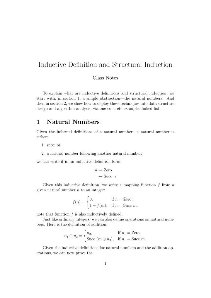
Inductive Definition and Structural Induction Class Notes To explain what are inductive definitions and structural induction, we start with, in section 1, a simple abstraction—the natural numbers. And then in section 2, we show how to deploy these techniques into data structure design and algorithm analysis, via one concrete example: linked list. 1 Natural Numbers Given the informal definitions of a natural number: a natural number is either: 1. zero; or 2. a natural number following another natural number. we can write it in an inductive definition form: n → Zero → Succ n Given this inductive definition, we write a mapping function f from a given natural number n to an integer: � 0 , if n = Zero; f ( n ) = 1 + f ( m ) , if n = Succ m. note that function f is also inductively defined. Just like ordinary integers, we can also define operations on natural num- bers. Here is the definition of addition: � if n 1 = Zero; n 2 , n 1 ⊕ n 2 = Succ ( m ⊕ n 2 ) , if n 1 = Succ m. Given the inductive definitions for natural numbers and the addition op- erations, we can now prove the 1

Thm 1: f ( n 1 ⊕ n 2 ) = f ( n 1 ) + f ( n 2 ) . Proof. Induction on n 1 . Case Zero left = f (Zero ⊕ n 2 ) = f ( n 2 ) . right = f (Zero) + f ( n 2 ) = 0 + f ( n 2 ) = f ( n 2 ) . Case Succ m left = f (Succ m ⊕ n 2 ) = f (Succ ( m ⊕ n 2 )) = 1 + f ( m ⊕ n 2 ) = 1 + f ( m ) + f ( n 2 ) . right = f (Succ m ) + f ( n 2 ) = 1 + f ( m ) + f ( n 2) . QED. By making use of addition, we can define multiplication on two natural numbers n 1 and n 2 : � Zero , if n 1 = Zero; n 1 ⊗ n 2 = n 2 ⊕ ( m ⊗ n 2 ) , if n 1 = Succ m. It is left an exercise to prove that Thm 2: f ( n 1 ⊗ n 2) = f ( n 1) × f ( n 2) . As a final example, we define an equality testing function � on two natural numbers n 1 and n 2 :  Succ Zero , if n 1 = Zero ∧ n 2 = Zero;    Zero , if n 1 = Zero ∧ n 2 = Succ m ;  n 1 � n 2 = Zero , if n 1 = Succ m ∧ n 2 = Zero;    if n 1 = Succ s ∧ n 2 = Succ t.  s � t, It is also left as an exercise to prove Thm 3: f ( n 1 � n 2) = ( f ( n 1) = f ( n 2)) . 2

2 Linked List The real power of inductive definitions and structural induction is in that it can be used to define a rather large set of useful data structures, say, linked list, binary trees, red-black trees, and so on. In this section, we illustrate the main idea by studying an inductively defined linked list. Informal description: a linked list is either 1. an empty list without any data; or 2. a linked list with a head node, followed by another linked list. And write into inductive definition form: list → Empty → Cons ( T, list ) We can define a function f on list l : � 0 , if l = Empty; f ( l ) = 1 + f ( m ) , if l = Cons ( x, m ) . intuitively, f counts the length of the list l . To concatenate two lists l 1 and l 2 , we write another inductively defined function g : � if l 1 = Empty; l 2 , g ( l 1 , l 2 ) = Cons ( x, g ( m, l 2 )) , if l 1 = Cons ( x, m ) . Intuitively, list concatenation does not change the list length, this fact is represented by Thm 4: f ( g ( l 1 , l 2 )) = f ( l 1 ) + f ( l 2 ) . Proof. By induction on l 1 . Case Empty left = f ( g (Empty , l 2 )) = f ( l 2 ) . right = f (Empty) + f ( l 2 ) = f ( l 2 ) . 3

Case Cons ( x, m ) left = f ( g (Cons ( x, m ) , l 2 )) = f (Cons ( x, g ( m, l 2 ))) = 1 + f ( g ( m, l 2 )) = 1 + f ( m ) + f ( l 2 ) right = f (Cons ( x, m )) + f ( l 2 ) = 1 + f ( m ) + f ( l 2 ) . QED. As a final example, if we reverse a linked list by function f : � Empty , if l = Empty; h ( l ) = g ( h ( m ) , Cons ( x, Empty)) , if l = Cons ( x, m ) . then we can prove Thm 5: f ( h ( l )) = f ( l ) . Proof left to you. 4