Imposing Hard Constraints on Deep Networks: Promises and - PowerPoint PPT Presentation
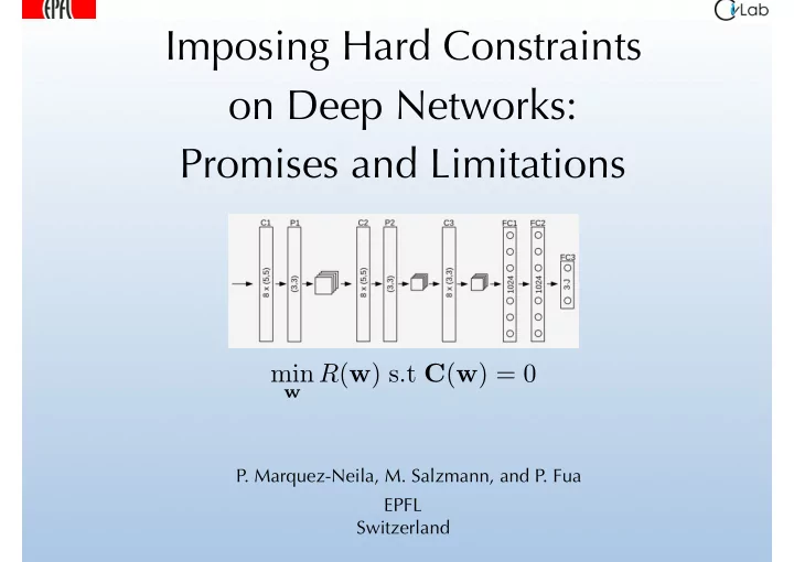
Imposing Hard Constraints on Deep Networks: Promises and Limitations min w R ( w ) s.t C ( w ) = 0 P. Marquez-Neila, M. Salzmann, and P. Fua EPFL Switzerland Motivation: 3D Pose Estimation Given a CNN trained to predict the 3D locations of
Imposing Hard Constraints on Deep Networks: Promises and Limitations min w R ( w ) s.t C ( w ) = 0 P. Marquez-Neila, M. Salzmann, and P. Fua EPFL Switzerland
Motivation: 3D Pose Estimation Given a CNN trained to predict the 3D locations of the person’s joints: • Can we increase precision by using our knowledge that her left and right limbs are of the same length? • If so, how should such constraints be imposed? 2
In Shallower Times V = 75 40 Reconstruction Error Yao11 Ours 30 20 10 50 100 150 200 250 N V = 75 Constraint Violation Yao11 0.3 Ours 0.2 0.1 0 50 100 150 200 250 N Regression from PHOG features. Constraining a Gaussian Latent Variable Model to preserve limb lengths: • Better constraint satisfaction without sacrificing accuracy. • Can this be repeated with CNNs? 3 Varol et al. CVPR’12
Standard Formulation Given • Deep Network architecture φ ( · , w ), • a training set S = { ( x i , y i ) , 1 ≤ i ≤ N } of N pairs of input and output vectors, x i and y i , find w ∗ = arg min w R S ( w ) , with R S ( w ) = 1 X L ( φ ( x i , w ) , y i ) . N i 4
Adding Constraints Hard Constraints: k } |U| Given a set of unlabeled points U = { x 0 k =1 , find min w R S ( w ) s.t C jk ( w ) = 0 ∀ j ≤ N C , ∀ k ≤ |U| , where C jk ( w ) = C j ( φ ( x 0 k ; w )). Soft Constraints: Minimize X ! X C jk ( w ) 2 min w R S ( w ) + λ j , j k where the λ j parameters are positive scalars that control the relative contribution of each constraint. In many “classical” optimization problems, hard constraints are preferred because they remove the need to adjust the values. λ 5
Lagrangian Optimization Karush-Kuhn-Tucker (KKT) conditions: L ( w , Λ ) , with L ( w , Λ ) = R ( w ) + Λ T C ( w ) , min w max Λ Iterative minimization scheme: At each iteration w ← w + d w with " # − J T r ( w t ) T J T J + η I � � ∂ C d w = ∂ w − C ( w t ) ∂ C Λ 0 ∂ w —> When there are millions of unknown these linear systems are HUGE ! 6
Krylov Subspace Method Solve Bv = b when the dimension of v so large that B cannot be stored in memory. • Solve linear system by iteratively finding approximate solutions in the subspace spanned by { b , Bb , B 2 b , ..., B k b } for k = 0 , 1 , ..., N • Use Pearlmutter Trick to compute terms of the form v T ∂ f ∂ w and v T ∂ f ∂ w —-> It can be done! 7
Results No Constraints 5.5 Soft-SGD ( = 10, = 1e 07, hm = 1) Soft-SGD ( = 1, = 1e 06, hm = 1) Soft-SGD ( = 1, = 1e 07, hm = 1) 5.0 Soft-Adam ( = 1, hm = 0) Soft-Adam ( = 10, hm = 0) Hard constraints help … Soft-Adam ( = 100, hm = 0) 4.5 Soft-Adam ( = 1, hm = 1) Soft-Adam ( = 10, hm = 1) Median constraint violation (mm) Soft-Adam ( = 100, hm = 1) 4.0 Hard-SGD ( = 10000, subiters= 1, hm = 1) Hard-SGD ( = 100000, subiters= 5, hm = 0) Hard-SGD ( = 100000, subiters= 5, hm = 1) 3.5 Hard-Adam (subiters= 1, hm = 1) Hard-Adam (subiters= 5, hm = 1) 3.0 Hard Constraints … but soft constraints help even more! 2.5 2.0 1.5 1.0 68 69 70 71 72 73 74 75 76 Soft Constraints Prediction error (mm) 8
Synthetic Example Let x and c i for 1 i 200 be vectors of dimension d and let w ∗ be either 1 2 k w � x 0 k 2 s.t k w � c i k � 10 = 0 , 1 i 200 min (Hard Constraints) w or 1 2 k w � x 0 k 2 + λ ( k w � c i k � 10) 2 X min (Soft Constraints) w 1 ≤ i ≤ 200 x 0 d = 1 e 6 d = 1 e 6 d = 2 All constraints active With constraint batches 9
Computational Complexity At each iteration: " # − J T r ( w t ) T J T J + η I � � ∂ C d w = ∂ w − C ( w t ) ∂ C Λ 0 ∂ w • Np is the size of a minibatch, which can be adjusted. • Nc is the number of constraints, which is large if they are all active. 10
Interpretation Hard constraints can be imposed on the output of Deep Nets but they are no more effective than soft ones: • Not all constraints are independent from each other, which results in ill-conditioned matrices. • We impose constraints on batches of constraints, which means we do not keep a consistent set of them. —> We might still present this work at a positive result workshop. 11
Low Hanging Fruits Typical approach: • Identify an algorithm that can be naturally extended. • Perform the extension. • Show that your ROC curve is above the others. • Publish in CVPR or ICCV. • Iterate. 12
Shooting for the Moon We choose to go to the Moon in this decade and do the other things, not because they are easy, but because they are hard. J.F. Kennedy, 1962 In the context of Deep Learning: • What makes Deep Nets tick? • What are their limits? • Can they be replaced by something more streamlined? 13
Recommend
More recommend
Explore More Topics
Stay informed with curated content and fresh updates.

