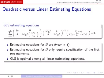
Implementing GLS Recall the assumptions of Approach 9: E( Y | x ) = - PowerPoint PPT Presentation

ST 762 Nonlinear Statistical Models for Univariate and Multivariate Response Implementing GLS Recall the assumptions of Approach 9: E( Y | x ) = f ( x , β ) , var( Y | x ) = σ 2 g ( β , θ , x ) 2 . Here: β is, as before, the vector of parameters in the mean function; θ is a possible additional parameter in the structure of the variance function; σ 2 is an additional dispersion parameter. 1 / 17

ST 762 Nonlinear Statistical Models for Univariate and Multivariate Response Ad hoc estimation scheme: Get initial estimate of β using OLS; i Get initial estimate of θ , if needed, and construct initial ii estimated weights 1 w j = ˆ � 2 � β OLS , ˆ ˆ g θ , x iii Re-estimate β using WLS, treating ˆ w j as fixed: solve the estimating equation n � w j { Y j − f ( x j , β ) } f β ( x j , β ) = 0 . ˆ j =1 2 / 17

ST 762 Nonlinear Statistical Models for Univariate and Multivariate Response Digression Gauss-Newton method for WLS (including OLS): The equation n � w j { Y j − f ( x j , β ) } f β ( x j , β ) = 0 . j =1 generally cannot be solved in closed form. But if β ∗ is close to the solution β , f ( x j , β ) ≈ f ( x j , β ∗ ) + f β ( x j , β ∗ ) T ( β − β ∗ ) , f β ( x j , β ) ≈ f β ( x j , β ∗ ) + f ββ ( x j , β ∗ ) ( β − β ∗ ) 3 / 17

ST 762 Nonlinear Statistical Models for Univariate and Multivariate Response Omitting terms likely to be small, the WLS estimating equation becomes � � n � w j f β ( x j , β ∗ ) f β ( x j , β ∗ ) T ( β − β ∗ ) j =1 n � ≈ w j { Y j − f ( x j , β ∗ ) } f β ( x j , β ∗ ) j =1 4 / 17

ST 762 Nonlinear Statistical Models for Univariate and Multivariate Response Write  f β ( x 1 , β ) T  . . X ( β ) =  .    ( n × p ) f β ( x n , β ) T   f ( x 1 , β ) . . f ( β ) =   .   ( n × 1) f ( x n , β )   w 1 0 0 . . . 0 w 2 0  . . .  ( n × n ) = W  . . .  ... . . .   . . .   0 0 w n . . . 5 / 17

ST 762 Nonlinear Statistical Models for Univariate and Multivariate Response Then the approximate equation may be written � X ( β ∗ ) T WX ( β ∗ ) � ( β − β ∗ ) ≈ X ( β ∗ ) T W { Y − f ( β ∗ ) } or (if the inverse exists) � − 1 X ( β ∗ ) T W { Y − f ( β ∗ ) } β ≈ β ∗ + � X ( β ∗ ) T WX ( β ∗ ) Iterative solution: β ( a +1) = β ( a ) + �� − 1 � T WX � T W � � � � � � �� Y − f X β ( a ) β ( a ) X β ( a ) β ( a ) Note that W is fixed throughout the inner circle of iteration. 6 / 17

ST 762 Nonlinear Statistical Models for Univariate and Multivariate Response Note that if the iteration converges, β ( a ) → β ( ∞ ) , and � T WX � � � X β ( a ) β ( a ) converges to a non-singular matrix, then � T W � � � �� Y − f = 0 X β ( ∞ ) β ( ∞ ) which is the original estimating equation written in matrix form. That is, the limit β ( ∞ ) does solve the original WLS problem. This algorithm, suitably refined, is the default method in both R’s nls() and SAS’s proc nlin . 7 / 17

ST 762 Nonlinear Statistical Models for Univariate and Multivariate Response Instead of the nested iterations, we could solve the last equation directly. Note This is not equivalent to minimizing n 1 � g ( β , θ , x j ) 2 { Y j − f ( x j , β ) } 2 , S g ( β ) = j =1 because differentiating S g ( β ) w.r.t. β also brings in the derivative of g ( · ). 8 / 17

ST 762 Nonlinear Statistical Models for Univariate and Multivariate Response The equation can be solved by a Gauss-Newton method; a similar approximation leads to the iteration β ( a +1) = β ( a ) + �� − 1 � T W ( a ) X � T W ( a ) � � � � � � �� Y − f X β ( a ) β ( a ) X β ( a ) β ( a ) where the weight matrix W is now updated using the current value of β ( a ) . That is, the weights are updated within the iteration, instead of being held constant, as in the WLS iteration; a nonlinear instance of Iteratively Reweighted Least Squares, IRWLS (note the redundancy!) or IWLS. 9 / 17

ST 762 Nonlinear Statistical Models for Univariate and Multivariate Response Estimating σ 2 By analogy with WLS, the natural estimator of σ 2 is either �� 2 � � x j , ˆ Y j − f n β GLS 1 � � 2 n � ˆ g β GLS , θ , x j j =1 or �� 2 � � x j , ˆ Y j − f n β GLS 1 � . � 2 n − p � ˆ g β GLS , θ , x j j =1 10 / 17

ST 762 Nonlinear Statistical Models for Univariate and Multivariate Response For fixed weights, the latter is unbiased. For fixed weights and Gaussian Y , the former is ML and the latter is REML. The latter is reported by most software. 11 / 17

ST 762 Nonlinear Statistical Models for Univariate and Multivariate Response Summary Model E( Y | x ) = f ( x , β ) , var( Y | x ) = σ 2 g ( β , θ , x ) 2 . Generalized least squares (GLS) n � w j { Y j − f ( x j , β ) } f β ( x j , β ) = 0 . j =1 12 / 17

ST 762 Nonlinear Statistical Models for Univariate and Multivariate Response Motivation Loss function n � w j { Y j − f ( x j , β ) } 2 , S g ( β ) = j =1 with plugged-in weights w j = g ( β , θ , x j ) − 2 . Gaussian distribution with mean f ( x j , β ) and plugged-in weights w j . 13 / 17

ST 762 Nonlinear Statistical Models for Univariate and Multivariate Response Implementations 3-step GLS (0) Get initial estimate ˆ β 1 Repeat until convergence, or for a fixed number of C steps: 2 ( t ) , x ) − 2 w j = g (ˆ Update the weights ˆ β 1 Estimate β using WLS: 2 Repeat until convergence β ( a +1) = β ( a ) + �� − 1 � � T � T � � � � � �� X WX X W Y − f β ( a ) β ( a ) β ( a ) β ( a ) ( t +1) Update the estimate ˆ β 3 14 / 17

ST 762 Nonlinear Statistical Models for Univariate and Multivariate Response Comment There are 2 loops In the inner loop (step 2.2), the weight matrix W is fixed 15 / 17

ST 762 Nonlinear Statistical Models for Univariate and Multivariate Response Implementations (continued) Iteratively reweighted least squares (IRWLS) (0) Get initial estimate ˆ β 1 Repeat until convergence: 2 ( t ) , x ) − 2 w j = g (ˆ Update the weights ˆ β 1 Estimate β using WLS 2 β ( a +1) = β ( a ) + �� − 1 � � T � T � � � � � �� X β ( a ) W ( a ) X β ( a ) X β ( a ) W ( a ) Y − f β ( a ) ( t +1) Update the estimate ˆ β 3 16 / 17

ST 762 Nonlinear Statistical Models for Univariate and Multivariate Response Comment There is only 1 loop The weight matrix W is iteratively updated 17 / 17