Impact of different levels of quadratic convex reformulation for - PowerPoint PPT Presentation

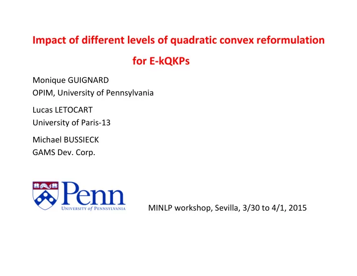
Impact of different levels of quadratic convex reformulation for E-kQKPs Monique G UIGNARD OPIM, University of Pennsylvania Lucas L ETOCART University of Paris-13 Michael BUSSIECK GAMS Dev. Corp. MINLP workshop, Sevilla , 3/30 to 4/1, 2015

Xiaoling Sun passed away April 24, 2014. He was here for the Seville MINLP workshop in 2010. This talk owes a lot to his work.

Quadratic Convex Reformulations   n Max { ( ) f x s t . . x X x , {0,1 } } Replace (P)   n Max { ( ) g x s t . . x X x , {0,1 } } by (P’) where X is a polyhedron, f ( x ) and g ( x ) are quadratic functions of x binary and g is concave.

Quadratic Convex Reformulations (QCR)   n Max { ( ) f x s t . . x X x , {0,1 } } Replace (P)   n Max { ( ) g x s t . . x X x , {0,1 } } by (P ’ ) where X is a polyhedron, f ( x ) and g ( x ) are quadratic functions of x binary and g is concave (convex if you minimize) . Idea 1: replace f ( x ) by a concave function g ( x ) which coincides with f ( x ) at every x feasible for (P).

FOR A MIN PROBLEM: This shows an example with two convex functions of one variable that coincide for x=0 and for x=1, but with clearly different minima for x ∈ [0, 1]. y=g1(x) y=g2(x) 0 1

Quadratic Convex Reformulations (QCR)   n Max { ( ) f x s t . . x X x , {0,1 } } Replace (P)   n Max { ( ) g x s t . . x X x , {0,1 } } by (P ’ ) where X is a polyhedron, f ( x ) and g ( x ) are quadratic functions of x binary and g is concave. Idea 1: replace f ( x ) by a concave function g ( x ) which coincides with f ( x ) at every x feasible for (P). idea 2: choose g ( x ) such that the continuous relaxation bound from (P ’ ) is as tight as possible among all possible g of a certain type.

APPLIED TO E-kQKP QKP: quadratic knapsack problem E-kQKP: quadratic knapsack problem with a cardinality constraint

Problem ( E − kQKP ) Formulation Formulation Mathematical formulation  n n � �  max f ( x ) = c ij x i x j      i = 1 j = 1       � n  j = 1 a j x j ≤ b (1) s.t. (E-kQKP)    � n (2)  j = 1 x j = k         x j ∈ { 0 , 1 } j = 1 , . . . , n  without constraint 2 : the 0-1 quadratic knapsack problem ( QKP ) without constraint 1 : the k-cluster problem

Problem ( E − kQKP ) Formulation Formulation Notations n : number of items a j : weight of item j ( j = 1 , . . . , n ) b : capacity of the knapsack c ij : profit associated with the selection of items i and j ( i , j = 1 , . . . , n ) k : number of items to be filled in the knapsack Assumptions c ij ∈ N i , j = 1 , . . . , n , a j ∈ N j = 1 , . . . , n , b ∈ N max j = 1 ,..., n a j ≤ b < � n j = 1 a j k ∈ { 2 , . . . , k max }

− Complexity and experimental environment Complexity NP-hard problem : generalization of ( QKP ) and k -cluster problems Experimental environment Carried out on SMP partition of MAGI using 30 cores Xeon 2 GHz with 500 GB of RAM CSDP integrated into COIN-OR for solving SDP programs IBM-CPLEX 12.4 : standard solver (with default settings) Average values over 10 instances n ∈ { 10 , 20 , . . . , 200 } k ∈ [ 1 , n / 4 ] , b ∈ [ 50 , 30 k ] , a j , c ij ∈ [ 1 , 100 ] Lucas L´ etocart (LIPN) Multithread et OC JCS P13 6 / 57

Quadratic Convex Reformulations   n Replace (P) Max { ( ) f x st . . x X , x {0,1 } }   n by (P') Max { ( ) g x s t . . x X , x {0,1 } }     where f x and g x are quadratic functions of x binary   and g x is concave of the form   g x ( ) f x ( ) w x ( )  where ( ) w x 0 whenever is feasible for (P). x

PRIOR PROGRESSIVE IMPROVEMENTS: Hammer and Rubin: eigenvalue method to get a uniform diagonal modification. Alain Billionnet, Sourour Elloumi: solve an SDP problem to get the best diagonal modifications. Alain Billionnet, Sourour Elloumi, MC Plateau: solve an SDP problem to get the best entire matrix modification using equality constraints if any . Shuhui Ji, Xiaojin Zheng and Xiaoling Sun: extension of the whole matrix modification .

− Quadratic Convex Reformulation (QCR) : a two-phase method [Billionnet, Elloumi and M-C. Plateau, Discrete Applied Mathematics, 2009] Phase 1 : Reformulate the objective function f ( x ) into an equivalent 0-1 program with a concave quadratic objective function f u ,α ( x ) depending on two parameters u and α both in R n . → an equivalent convex 0-1 program Phase 2 : Apply a standard 0-1 convex quadratic solver to this new problem. QCR - Phase I : Addition of two functions null on the feasible set n x 2 � � � q u ( x ) = u i i − x i i = 1 � 2 � � � n n n q α ( x ) = � α i x i � x j − k q v ( x ) = v � x j − k or i = 1 j = 1 j = 1

− QCR : A two-phase method QCR - Phase I : Reformulation 1 New objective function (concave iff quadratic terms matrix is SDP) :   n n n � � � � x 2 � f u ,α ( x ) = f ( x ) − i − x i − α i x i x j − k u i   i = 1 i = 1 j = 1 Reformulation 2 [Faye, Roupin, 4OR, 2007 ; Billionnet, Elloumi and Lambert, Math. Prog., 2009] 2   n n � � � x 2 � f u , v ( x ) = f ( x ) − i − x i − v x j − k u i   i = 1 j = 1 identical bounds consumes the least amount of computation times

introduce new variables X to replace the products x x , do not write ij i j  X x x because it is nonlinear, but add constraints that come from the ij i j definition of these new variables ( X is viewed as a matrix ) defined by   x x x x 1 1 1 n     = xx T X      x x x x n 1 n n  X is of rank 1 (ignore) this implies that  X - xx T = 0 (still nonlinear !) therefore relax as X - xx T 0 (nonlinear, or equivalently (*))   T 1 x   0   x X    2 X ( ) x x ii i i

________________________________________________________ (*) Schur’s lemma says that   A y    1   0 C xA y 0   x C ________________________________________________________

− QCR : A two-phase method Best values for the parameters u ∈ R n and v ∈ R Solve the semi-definite relaxation of the problem ( E − kQKP ) :  � n � n max j = 1 c ij X ij i = 1       X ii = x i i = 1 , . . . , n ( u ∗ )  s.t.        n n n   x j = − k 2 � � � ( v ∗ )  X ij − 2 k    i = 1 j = 1 j = 1       � n ( SDP ) j = 1 a j x j ≤ b     � n j = 1 x j = k       � 1   x t  �   � 0   x X         x ∈ R n , X ∈ R n × n  Lucas L´ etocart (LIPN) Multithread et OC JCS P13 9 / 57

− An improved convex 0-1 quadratic reformulation for ( E − kQKP ) (1/4) [S. Ji, X. Zheng and X. Sun, Pacific Journal of Optimization, 2012] From f ( x ) = x t Cx Consider the decomposition of f ( x ) f ( x ) = x t ( C − M ) x + x t Mx , where C − M � 0 and M = Diag ( u ) + P + N with u ∈ R n , P ∈ R n × n and N ∈ R n × n + −

− An improved convex 0-1 quadratic reformulation for ( E − kQKP ) (2/4) f ( x ) = x t ( C − Diag ( u ) − P − N ) x + x t ( Diag ( u ) + P + N ) x = x t ( C − Diag ( u ) − P − N ) x + u t x + � n i , j = 1 [ P ij x i x j + N ij x i x j ] = x t ( C − Diag ( u ) − P − N ) x + u t x + � n i , j = 1 [ P ij s ij − N ij t ij ] where s ij = min ( x i , x j ) , t ij = − max ( 0 , x i + x j − 1 ) ( x i x j = min ( x i , x j ) = max ( 0 , x i + x j − 1 ) for any x i , x j ∈ { 0 , 1 } )

− An improved convex 0-1 quadratic reformulation for ( E − kQKP ) (3/4) Relax s ij = min ( x i , x j ) to two linear inequalities s ij ≤ x i and s ij ≤ x j and t ij = − max ( 0 , x i + x j − 1 ) to t ij ≤ 0 and t ij ≤ 1 − x i − x j . without affecting the optimal solution of the problem. The reformulation is equivalent to the convex 0-1 quadratic program :  f ( x ) = x t ( C − Diag ( u ) − P − N ) x + u t x + � n i , j = 1 [ P ij s ij + N ij t ij ] max   � n  s.t. j = 1 a j x j ≤ b     � n j = 1 x j = k  s ij ≤ x i , s ij ≤ x j i , j = 1 , . . . , n    t ij ≤ 0 , t ij ≤ 1 − x i − x j i , j = 1 , . . . , n     x j ∈ { 0 , 1 } j = 1 , . . . , n 

− An improved convex 0-1 quadratic reformulation for ( E − kQKP ) (4/4) The optimal parameters ( u ∗ , v ∗ , P ∗ , N ∗ ) can be found by solving a SDP :  � n � n max j = 1 c ij X ij i = 1       X ii = x i i = 1 , . . . , n ( u ∗ )  s.t.        n n n   x j = − k 2 � � � i = 1 , . . . , n ( v ∗ ) X ij − 2 k     i = 1 j = 1 j = 1   � n  j = 1 a j x j ≤ b         � n j = 1 x j = k    (1 and 2)  i , j = 1 , . . . , n ( P ∗ ) X ij ≤ x i , X ij ≤ x j        (3 and 4)  X ij ≥ x i + x j − 1 , X ij ≥ 0 i , j = 1 , . . . , n ( N ∗ )       � 1   x t �   � 0   x X         x ∈ R n , X ∈ S n 