Hypothesis Testing Appendix James J. Heckman University of Chicago - PowerPoint PPT Presentation
Hypothesis Testing Appendix James J. Heckman University of Chicago Econ 312 Spring 2019 A Further results on Bayesian vs. Classical Testing (The phenomenon shows up even when we dont have .) Point mass placed at 0 ; 0
Hypothesis Testing Appendix James J. Heckman University of Chicago Econ 312 Spring 2019
A Further results on Bayesian vs. Classical Testing (The phenomenon shows up even when we don’t have � � � .) Point mass placed at � 0 ; � 0 For rest of parameter space, we have 1 � � 0 = � 1 ; � 1 is density of � � ( � | � ) is model. 1
Marginal density of � = Z � ( � ) = � ( � | � ) � � ( � ) = � ( � | � 0 ) � 0 + (1 � � 0 ) � 1 ( � ) Z � 1 ( � ) = � ( � | � ) � 1 ( � ) �� 2
Posterior probability that � = � 0 is � ( � | � 0 ) � 0 � ( � 0 | � ) = � ( � ) � ( � | � 0 ) � 0 = � ( � | � 0 ) � 0 + (1 � � 0 ) � 1 ( � ) 1 = 1 + (1 � � 0 ) � 1 ( � ) � ( � | � 0 ) � 0 3
� The posterior probability that for � 0 1 Posterior Odds Ratio = μ 1 � � 0 ¶ � 1 ( � ) � ( � | � 0 ) � 0 μ ¶ μ � ( � | � 0 ) ¶ � 0 = 1 � � 0 � 1 ( � ) Bayes factor: � ( � | � 0 ) � 1 ( � ) 4
� � � � � � � � � � � � � � � � � � � � � Example: Let � � � ( �� � 2 ) ; � 2 known. ¸ ¡ ¯ ¢ 1 ¡ ¢ 2 � � ¯ �� � 2 �� L � � = exp p � � 2 � 2 2 �� 2 �� Let � 1 = � ( � 1 � � 2 ) be prior; then � 1 = � ( �� � 2 + � 2 �� ) ¸ � 1 h ³ ´i � 1 2 2 exp � ( ¯ � � � ) � 2 + � 2 2 � � 2 + � 2 � 1 + 1 � � 0 2 � ( � 0 | � ) = · ¸ 2 ¡ ¢ � 1 � ( ¯ � � � 0 ) 2 exp � 0 2 � � 2 � 2 2 center at � = � 0 . (This is a judgment about priors.) 5
� � � � � � � � � h i � 1 � 1 � 2 exp � 1 + (1 � � 0 ) 2[1+ � 2 � ( �� 2 )] � ( � 0 | � ) = (1 + �� 2 �� 2 ) 1 � 2 � 0 As � � � we get “Lindley Paradox” ¯ ¯ ¯ ¯ ¯ � � � 0 � = ³ ´ usual normal statistic (2 tail test). 6
Look at the following table of values: � ( � 0 | � ) , � = � 0 , � 0 = 1 � 2 , � = � . � (sample size) � score � value 1 5 10 20 50 100 1000 1.645 .1 .42 .44 .49 .56 .65 .72 .89 1.960 .05 .35 .33 .37 .42 .52 .60 .80 2.576 .01 .21 .13 .14 .16 .22 .27 .53 3.291 .001 .086 .026 .024 .026 .034 .045 .124 Observe: Not monotone in � : 7
� Now, consider the minimum of � ( � 0 | � ) over all � ; and � 1 = (marginal on alternative) Thm (Dickey and Savage): ¸ � 1 1 + (1 � � 0 ) � ( � ) � ( � 0 | � ) = � ( � | � 0 ) � 0 where � ( � ) = sup � ( � | � ) � 6 = � 0 usually obtained by substituting in maximum likelihood esti- mate. 8
The bound on the Bayes factor is � = � ( � | � 0 ) � � ( � | � 0 ) . � 1 ( � ) � ( � ) The proof of this is really trivial. 9
� � � � Now, look at the example (MLE): ¡ ¯ ¢ � | ¯ � ( � ) = � � ( � 0 | � ) " # � 1 (2 �� 2 �� ) � 1 1 + 1 � � 0 2 ¡ ¯ ¢ 2 � (2 � 2 �� ) (2 �� 2 �� ) � 1 2 exp � � 0 � � � 0 μ 1 ¶¸ � 1 1 + 1 � � 0 2 � 2 = exp � 0 For � 0 = 1 2 we get that for � � 1 � 68 (Berger and Selke; JASA , 1987). 10
� � ( � 0 | � ) � [ � ( value )] × [1 � 25 � ] . � values Lower bound on Bound on Bayes factor � ( � 0 | � ) 1.645 .1 .205 1/(3.87) 1.960 .05 .127 1/(6.83) 2.576 .01 .035 1/(27.60) 3.291 .001 .0044 1/(224.83) 11
� Thm. Berger and Selke. ½ ¾ � 1 is symmetric about � 0 � = � 1 : and non-increasing in | � � � 0 | � values Lower bound on Bound on Bayes factor � ( � 0 | � ) 1.645 .1 .390 1/(1.56) 1.960 .05 .290 1/(2.45) 2.576 .01 .109 1/(8.17) 3.291 .001 .018 1/(54.55) 12
� � B Bayesian Credibility Sets Def. A 100 (1 � � ) % credible set for � is a subset � of � such that Z d � � ( � | � ) ( � ) 1 � � � � ( � | � ) = Z = � ( � | � ) d � . 13
What is “best” ratio? A 100 (1 � � ) % highest posterior density credible set is a subset C of � such that � = { � | � ( � | � ) � � ( � ) } where � ( � ) is the largest constant such that � ( � | � ) � 1 � � . 14
� Example. Let � ( � | � ) = � ( � ( � ) � � 2 ) be a posterior 100 (1 � � ) % credible set is given by ³ � ( � ) + � � 1 ³ � ´ �� � ( � ) � � � 1 ³ � ´ ´ , 2 2 identical to the classical case for normal posteriors. Consider, however, what would happen in the Dickey Leamer � case. A possibility of disconnected credibility sets (multimodel). This can happen in the classical case. 15
�� �� � Problems. The forms of credible sets are not subject to simple ends. Example. Suppose the posterior is � ( � | � ) = � � 0 1 + � 2 ¡ 1 + � 2 ¢ ln � ( � | � ) = ln � + � � ln � ln � ( � | � ) 2 � = 1 � 1 + � 2 16
� � 2 ln � ( � | � ) 1 + � 2 + (2 � ) (2 � ) 2 = ¡ 1 + � 2 ¢ 2 �� 2 � 2 � 2 ¸ 2 = 1 + � 2 � 1 1 + � 2 ¸ � � 2 � 1 2 = � 0 , 1 + � 2 1 + � 2 where � � 1 . This is increasing in � . � credible set is ( � ( � ) � � ) . 17
� � Use a transformation: = exp ( � ) ¡ 1 + (log � ) 2 ¢ � 1 � ( � ) = decreasing on (1 � exp ( � )) . � we have a credible set given by (1 � d ( � )) , and in terms of the original coordinate system, by (0 � ln d ( � )) (upper tail in original parametrization, lower tail in new para- metrization). 18
� � � � � � C Model Selection in Bayesian Way The common classical approach is to use a pretest procedure. We seek � ( � | � ) , � = �� + � , � � � (0 � � � 1 � � ) . Predictive density under the hypothesis: Z Z � ( � | � ) = � ( � | �� � ) � ( �� � ) �� �� , � ( � | � ) = � ( � | � ) � ( � ) ¡ � � ; ( � � ) � 1 ¢ Prior � ( � ) : ¡ �� � � � � 1 � + � ( � � ) � 1 � 0 ¢ where we assume that � is known. 19
�� � � 1 � � + � ( � � ) � 1 � 0 � ( � ) = μ ¶ � 1 (2 � ) � 1 2 | � ( � ) | � 1 2 exp � ( � ) = 2 �� ( � � �� � ) 0 � � 1 ( � � �� � ) = 20
� � Let � � = � � 1 � � . £ ¤ � 1 � � 1 ( � ) � ( � � ) � 1 � 0 + � � 1 � � = h � � � � ( � 0 � + � � ) � 1 � 0 i = � � | � � + � 0 � | � 1 | � ( � ) | � 1 = ˆ � = ( � 0 � ) � 1 � 0 � � 0 � = 21
� � � � � � � � � Exercise. Prove that ³ ´ 0 ³ ´ � � � ˆ � � � ˆ = ³ � � � � ´ ¡ ( � � ) � 1 + � � 1 ¢ � 1 ³ � � � � ´ ˆ ˆ + ( � � �� � ) 0 ( � � �� � ) = ³ � � � � ´ ³ � � � � ´ � ( � � + � ) � 1 � ˆ ˆ . For the case when � � 1 is unknown (gamma-normal case), ¡ � | � � � � � 1 ( � � ) � 1 ¢ ( �� � ) ¡ ¢ � | � 2 . 1 � � 1 22
� � Then, as shown, we have predictive density: Z Z � ( � ) = · · · � ( � | �� � ) � ( �� � ) �� �� ¯ ¯ 2 μ ¶ � � 1+ � 1 ¯ ¯ 2 ¯ ¯ = � ( � 1 � � ) � 1 + � ¯ ¯ � 2 � 2 1 � � � � ( � � + � 0 � ) � 1 � 0 = | � � | | � � + � 0 � | � 1 | � | = ( � 1 ) � 1 � 2 ¡ � 1 ¢ 2 + � 2 � 1 ! � ( � 1 � � ) = � �� 2 ¡ � 1 ¢ 2 � 1 ! 23
� � � � �� � � � The Bayes factor for � � relative to � � is 1 � � � | � 1 � + � 0 � ( � 1 � � � ) | � � � | | � � 2 2 ¯ ¯ ¯ ¯ 1 ¯ � 1 � ( � 1 � � � ) ¯ � � ¯ ¯ � � � + � 0 2 2 ³ ´ � ( � 1 � + � ) 2 � 1 � + � � � 2 1 � 1 � · � � � . ³ ´ � ( � 1 � + � ) 1 � 2 � �� + � � � 2 24
� � � � � � � � �� � D Di � use Prior Approach 1 Let | � � � | 2 , � = �� � , get small and set � 1 = 0 (in which case we don’t get ). What types of di � use priors? (Many exist and they do not all lead to the same inference – a problem.) = or = ( � ) or 2 � � 2 � 0 � , = ( � ) and set � � 0 . This is like saying we don’t have many a priori observations! 25
�� �� � � � ¯ ¯ μ ESS � ¶ � 1 ¯ � 0 ¯ 2 � � ( � | � � ) 2 , 2 � 2 1 � ( � | � � ) � � ESS � | � 0 � � � | 2 where ESS is the ��� regression sum of squares. 26
� � � This strongly favors a small parameter model, ¯ ¯ μ ESS � ¶ � 1 ¯ � 0 ¯ 2 2 = 1 ESS � | � 0 � � � | 2 or μ ESS � ¶ � 2 = . ESS � There is no unique di � use prior. 27
� � � � � E Dominated Priors and ��� As � , � , and � 0 � grow, ¯ ¯ μ ESS � ¶ � 1 ¯ � 0 ¯ 2 � ( � | � � ) 2 � ( � | � � ) = � . 1 ESS � | � 0 � � � | 2 � � � , to derive ��� , assume,: X � 0 � 28
Recommend
More recommend
Explore More Topics
Stay informed with curated content and fresh updates.
