HW1 Grades our out Total: 180 Min: 55 Max: 188(178+10 for bonus - PowerPoint PPT Presentation
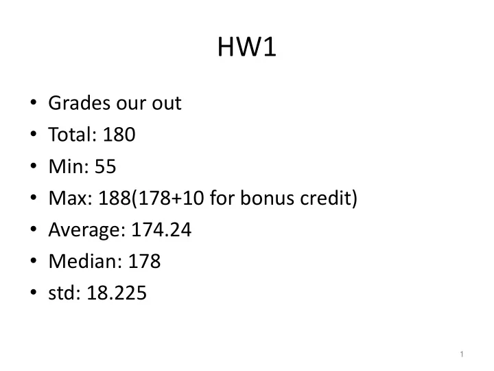
HW1 Grades our out Total: 180 Min: 55 Max: 188(178+10 for bonus credit) Average: 174.24 Median: 178 std: 18.225 1 Top5 on HW1 1. Curtis, Josh (score: 188, test accuracy: 0.9598) 2. Huang, Waylon (score: 180, test
HW1 • Grades our out • Total: 180 • Min: 55 • Max: 188(178+10 for bonus credit) • Average: 174.24 • Median: 178 • std: 18.225 1
Top5 on HW1 1. Curtis, Josh (score: 188, test accuracy: 0.9598) 2. Huang, Waylon (score: 180, test accuracy: 0.8202) 3. Luckey, Royden (score: 180, test accuracy: 0.8192) 4. Luo, Mathew Han (score: 180, test accuracy: 0.8174) 5. Shen, Dawei (score: 180, test accuracy: 0.8130) 2
CSE446: Ensemble Learning - Bagging and Boosting Spring 2017 Ali Farhadi Slides adapted from Carlos Guestrin, Nick Kushmerick, Padraig Cunningham, and Luke Zettlemoyer
4
5
Voting (Ensemble Methods) • Instead of learning a single classifier, learn many weak classifiers that are good at different parts of the data • Output class: (Weighted) vote of each classifier – Classifiers that are most “sure” will vote with more conviction – Classifiers will be most “sure” about a particular part of the space – On average, do better than single classifier! • But how??? – force classifiers to learn about different parts of the input space? different subsets of the data? – weigh the votes of different classifiers?
BAGGing = Bootstrap AGGregation (Breiman, 1996) • for i = 1, 2, …, K: – T i randomly select M training instances with replacement – h i learn(T i ) [Decision Tree, Naive Bayes, …] • Now combine the h i together with uniform voting (w i =1/K for all i)
8
decision tree learning algorithm; very similar to version in earlier slides 9
shades of blue/red indicate strength of vote for particular classification
Fighting the bias-variance tradeoff • Simple (a.k.a. weak) learners are good – e.g., naïve Bayes, logistic regression, decision stumps (or shallow decision trees) – Low variance, don’t usually overfit • Simple (a.k.a. weak) learners are bad – High bias, can’t solve hard learning problems • Can we make weak learners always good??? – No!!! – But often yes…
Boosting [Schapire, 1989] • Idea: given a weak learner, run it multiple times on (reweighted) training data, then let learned classifiers vote • On each iteration t : – weight each training example by how incorrectly it was classified – Learn a hypothesis – h t – A strength for this hypothesis – t • Final classifier: • Practically useful • Theoretically interesting
time = 0 blue/red = class size of dot = weight weak learner = Decision stub: horizontal or vertical li 14
time = 1 this hypothesis has 15% error and so does this ensemble, since the ensemble contains just this one hypothesis 15
time = 2 16
time = 3 17
time = 13 18
time = 100 19
time = 300 overfitting! 20
Learning from weighted data • Consider a weighted dataset – D(i) – weight of i th training example ( x i ,y i ) – Interpretations: • i th training example counts as if it occurred D(i) times • If I were to “resample” data, I would get more samples of “heavier” data points • Now, always do weighted calculations: – e.g., MLE for Naïve Bayes, redefine Count(Y=y) to be weighted count: – setting D(j)=1 (or any constant value!), for all j, will recreates unweighted case
Given: Initialize: How? Many possibilities. Will For t=1…T: see one shortly! • Train base classifier h t (x) using D t Why? Reweight the data: • Choose α t examples i that are misclassified will have • Update, for i=1..m: higher weights! with normalization constant: • y i h t (x i ) > 0 h i correct • y i h t (x i ) < 0 h i wrong • h i correct, α t > 0 D t+1 (i) < D t (i) Output final classifier: • h i wrong, α t > 0 D t+1 (i) > D t (i) Final Result: linear sum of “base” or “weak” classifier outputs.
Given: Initialize: For t=1…T: • Train base classifier h t (x) using D t • Choose α t • Update, for i=1..m: • ε t : error of h t , weighted by D t • 0 ≤ ε t ≤ 1 • α t : α t • No errors: ε t =0 α t =∞ • All errors: ε t = 1 α t =−∞ • Random: ε t = 0.5 α t =0 ε t
What t to choose for hypothesis h t ? [Schapire, 1989] Idea: choose t to minimize a bound on training error! Where
What t to choose for hypothesis h t ? [Schapire, 1989] Idea: choose t to minimize a bound on training error! Where This equality isn’t And obvious! Can be shown with algebra (telescoping sums)! If we minimize t Z t , we minimize our training error!!! • We can tighten this bound greedily, by choosing t and h t on each iteration to minimize Z t . • h t is estimated as a black box, but can we solve for t ?
Summary: choose t to minimize error bound [Schapire, 1989] We can squeeze this bound by choosing t on each iteration to minimize Z t . For boolean Y: differentiate, set equal to 0, there is a closed form solution! [Freund & Schapire ’97]:
Given: Initialize: For t=1…T: • Train base classifier h t (x) using D t • Choose α t • Update, for i=1..m: with normalization constant: Output final classifier:
Initialize: Use decision stubs as base classifier For t=1…T: Initial: • • Train base classifier h t (x) using D t D 1 = [D 1 (1), D 1 (2), D 1 (3)] = [.33,.33,.33] • t=1: Choose α t • Train stub [work omitted, breaking ties randomly] • h 1 (x)=+1 if x 1 >0.5, -1 otherwise • ε 1 =Σ i D 1 (i) δ (h 1 (x i )≠ y i ) = 0.33 × 1+0.33 × 0+0.33 × 0=0.33 • Update, for i=1..m: • α 1 =(1/2) ln((1- ε 1 )/ε 1 )=0.5 × ln(2)= 0.35 • D 2 (1) α D 1 (1) × exp(- α 1 y 1 h 1 (x 1 )) Output final classifier : = 0.33 × exp(-0.35 × 1 × -1) = 0.33 × exp(0.35) = 0.46 • D 2 (2) α D 1 (2) × exp(- α 1 y 2 h 1 (x 2 )) = 0.33 × exp(-0.35 × -1 × -1) = 0.33 × exp(-0.35) = 0.23 • D 2 (3) α D 1 (3) × exp(- α 1 y 3 h 1 (x 3 )) x 1 y = 0.33 × exp(-0.35 × 1 × 1) = 0.33 × exp(-0.35) =0.23 • D 2 = [D 1 (1), D 1 (2), D 1 (3)] = [0.5,0.25,0.25] -1 1 t=2 • Continues on next slide! x 1 0 -1 1 1 H(x) = sign(0.35 × h 1 (x)) • h 1 (x)=+1 if x 1 >0.5, -1 otherwise
• D 2 = [D 1 (1), D 1 (2), D 1 (3)] = [0.5,0.25,0.25] Initialize: t=2: For t=1…T: • Train stub [work omitted; different stub because of • Train base classifier h t (x) using D t new data weights D; breaking ties opportunistically • Choose α t (will discuss at end)] • h 2 (x)=+1 if x 1 <1.5, -1 otherwise • ε 2 =Σ i D 2 (i) δ (h 2 (x i )≠ y i ) = 0.5 × 0+0.25 × 1+0.25 × 0=0.25 • α 2 =(1/2) ln((1- ε 2 )/ε 2 )=0.5 × ln(3)= 0.55 • Update, for i=1..m: • D 2 (1) α D 1 (1) × exp(- α 2 y 1 h 2 (x 1 )) = 0.5 × exp(-0.55 × 1 × 1) = 0.5 × exp(-0.55) = 0.29 Output final classifier : • D 2 (2) α D 1 (2) × exp(- α 2 y 2 h 2 (x 2 )) = 0.25 × exp(-0.55 × -1 × 1) = 0.25 × exp(0.55) = 0.43 • D 2 (3) α D 1 (3) × exp(- α 2 y 3 h 2 (x 3 )) = 0.25 × exp(-0.55 × 1 × 1) = 0.25 × exp(-0.55) = 0.14 x 1 y • D 3 = [D 3 (1), D 3 (2), D 3 (3)] = [0.33,0.5,0.17] t=3 -1 1 • Continues on next slide! x 1 0 -1 1 1 H(x) = sign(0.35 × h 1 (x)+0.55 × h 2 (x)) • h 1 (x)=+1 if x 1 >0.5, -1 otherwise • h 2 (x)=+1 if x 1 <1.5, -1 otherwise
• D 3 = [D 3 (1), D 3 (2), D 3 (3)] = [0.33,0.5,0.17] Initialize: t=3: For t=1…T: • Train stub [work omitted; different stub • Train base classifier h t (x) using D t because of new data weights D; breaking ties • Choose α t opportunistically (will discuss at end)] • h 3 (x)=+1 if x 1 <-0.5, -1 otherwise • ε 3 =Σ i D 3 (i) δ (h 3 (x i )≠ y i ) = 0.33 × 0+0.5 × 0+0.17 × 1=0.17 • Update, for i=1..m: • α 3 =(1/2) ln((1- ε 3 )/ε 3 )=0.5 × ln(4.88)= 0.79 Output final classifier : • Stop!!! How did we know to stop? x 1 y -1 1 x 1 0 -1 1 1 H(x) = sign(0.35 × h 1 (x)+0.55 × h 2 (x)+0.79 × h 3 (x)) • h 1 (x)=+1 if x 1 >0.5, -1 otherwise • h 2 (x)=+1 if x 1 <1.5, -1 otherwise • h 3 (x)=+1 if x 1 <-0.5, -1 otherwise
Strong, weak classifiers • If each classifier is (at least slightly) better than random: t < 0.5 • Another bound on error: • What does this imply about the training error? – Will reach zero! – Will get there exponentially fast! • Is it hard to achieve better than random training error?
Boosting results – Digit recognition [Schapire, 1989] Test error Training error • Boosting: – Seems to be robust to overfitting – Test error can decrease even after training error is zero!!!
Boosting generalization error bound [Freund & Schapire, 1996] Constants: • T : number of boosting rounds – Higher T Looser bound • d : measures complexity of classifiers – Higher d bigger hypothesis space looser bound • m : number of training examples – more data tighter bound
Boosting generalization error bound [Freund & Schapire, 1996] Constants: Theory does not match practice : • • T : number of boosting rounds: • Robust to overfitting – Higher T Looser bound, what does this imply? • Test set error decreases even after training error is • d : VC dimension of weak learner, measures zero complexity of classifier Need better analysis tools • – Higher d bigger hypothesis space looser bound • we’ll come back to this later in the quarter • m : number of training examples – more data tighter bound
Recommend
More recommend
Explore More Topics
Stay informed with curated content and fresh updates.
