How to Model Quantum Plasmas Giovanni Manfredi Laboratoire de - PDF document
How to Model Quantum Plasmas Giovanni Manfredi Laboratoire de Physique des Milieux Ionis es et Applications CNRS and Universit e Henri Poincar e, Nancy, France Outline of the talk Introduction/Motivations When are quantum
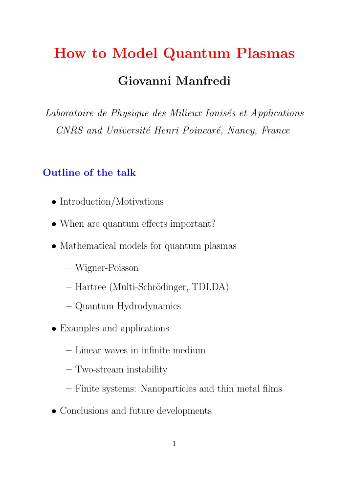
How to Model Quantum Plasmas Giovanni Manfredi Laboratoire de Physique des Milieux Ionis´ es et Applications CNRS and Universit´ e Henri Poincar´ e, Nancy, France Outline of the talk • Introduction/Motivations • When are quantum effects important? • Mathematical models for quantum plasmas – Wigner-Poisson – Hartree (Multi-Schr¨ odinger, TDLDA) – Quantum Hydrodynamics • Examples and applications – Linear waves in infinite medium – Two-stream instability – Finite systems: Nanoparticles and thin metal films • Conclusions and future developments 1
Introduction/Motivations Fundamental questions • How are kinetic equations modified by quantum effects? • What happens to typical plasma effects : Debye screening, Landau damping, plasma and sound waves . . . ? Applications • Semiconductors – Miniaturisation of electronic devices – De Broglie wavelength comparable to size of the device • Nanosized objects – E.g.: Metal clusters, thin metal films – Clusters composed of small (10 − 1000) number of metallic atoms – Valence electrons behave as an electron plasma, neutral- ized by ionic background – Large particle densities: n ∼ 10 28 m − 3 – But no crystalline structure: no Block waves etc . . . (“amorphous metals”) 2
When are quantum effects important? • Define the thermal de Broglie wavelength (“size” of a quan- tum particle): h ¯ λ B = mv th • Quantum effects are important when λ B exceeds the inter- particle distance d = n − 1 / 3 , i.e.: nλ 3 B > 1 • This condition corresponds to T < T F , where T F is the Fermi temperature: h 2 κT F = E F = mv 2 2 = ¯ 2 m (3 π 2 ) 2 / 3 n 2 / 3 F and E F and v F are the Fermi energy and Fermi speed. • We have obtained our first dimensionless parameter : 3 / 2 T F = nλ 3 χ ≡ B T 3
Collisionless (mean-field) regimes Classical plasmas ( T ≫ T F ): • The coupling parameter is defined as the ratio of the interac- tion energy to the kinetic energy g C ≡ E int E kin • For a classical plasma, the interaction and kinetic energies are given respectively by the electrostatic and the thermal energy: E int = e 2 n 1 / 3 ; E kin = κT ε 0 • The classical coupling parameter can be expressed as 2 / 3 = e 2 n 1 / 3 1 g c = nλ 3 ε 0 κT D where λ D = ( ε 0 κT/ne 2 ) 1 / 2 is the Debye length. • g C ≪ 1 ⇒ collective effects dominate (mean-field) g C ≃ 1 ⇒ two-body correlations (collisions) are important. • Classical plasmas are collisionless at high temperatures and low densities. 4
Quantum plasmas ( T ≪ T F ): • Typical time, velocity, and length scales in a quantum plasma: – Plasma frequency: 1 / 2 e 2 n ω p = mε 0 – Fermi velocity (replaces the classical thermal velocity; measures velocity dispersion): v F = ¯ h m (3 π 2 n ) 1 / 3 – Fermi length (length scale for electrostatic screening in a quantum plasma): λ F = v F ω p • The kinetic energy is given by the Fermi energy E kin = E F • The quantum coupling parameter becomes 2 / 3 2 = e 2 m g Q = E int 1 ¯ hω p n − 1 / 3 = = h 2 ε 0 nλ 3 E F E F ¯ F • Note: a quantum plasma is “more collisionless” at higher densities. 5
log T – log n diagram (for electrons) • We plot the three curves corresponding to T = T F , g C = 1, g Q = 1 6
log T – log n diagram (for electrons) • We plot the three curves corresponding to T = T F , g C = 1, g Q = 1 7
log T – log n diagram (for electrons) • We plot the three curves corresponding to T = T F , g C = 1, g Q = 1 NB: Metals (and metallic nanoparticles) fall in the strongly-coupled quantum region ( T < T F , g Q > 1): is the Wigner equation ap- propriate there? 8
Pauli blocking • The Pauli exclusion principle inhibits electron-electron colli- sions at low temperatures (collision rate: ν ee = 1 /τ ee ). • For T = 0, we have that: ν ee → 0 • For T < T F , only electrons with E F − κT < E < E F + κT can undergo collisions. • Their collision rate is: ν ′ ee ≃ κT/ ¯ h (Energy × lifetime ∼ ¯ h ). • The average e-e collision rate is obtained by multiplying ν ′ ee by the fraction of electrons that can collide ( ∼ T/T F ): = κT 2 ee × T ν ee = ν ′ T F hT F ¯ • In normalized units, this expression reads as: 2 2 ν ee = E F T 1 T = g 1 / 2 ω p hω p ¯ T F T F Q • Thus ν ee < ω p in the region where T < T F , g Q > 1. 9
Example with typical metallic parameters 5 × 10 28 m − 3 n T 300 K 1 . 3 × 10 16 s − 1 ω pe τ pe 0 . 5 fs 10 11 s − 1 ν ee 5 . 7 × 10 4 K T F 0 . 9 × 10 6 ms − 1 v F 0 . 9 × 10 − 10 m λ F g Q 13.5 • τ pe = 2 π/ω pe is of the order of the femtosecond • λ F is of the order of the ˚ Angstrom • The e-e collision frequency is small: ν ee ≪ ω pe Remark Far from thermodynamic equilibrium, Pauli blocking is less im- portant, and the collision frequency can be considerably larger. 10
Wigner-Poisson model • Representation of quantum mechanics in the classical phase space. Wigner function: m � + ∞ x + λ x − λ N h dλ ψ α e imvλ/ ¯ −∞ ψ ∗ f e ( x, v ) = h p α � α 2 π ¯ 2 2 α =1 � N with the probabilities p α satisfying α =1 p α = 1. • The Wigner function is not a true probability density, as it can be negative • Can be used to compute averages : � � � A � = f e ( x, v ) A ( x, v ) dxdv • The Wigner function obeys the following evolution equation: ∂f e ∂t + v∂f e ∂x + em x + λ x − λ dλ dv ′ e im ( v − v ′ ) λ/ ¯ − φ f e ( x, v ′ , t ) = 0 � � h φ h 2 2 iπ ¯ 2 2 coupled to Poisson’s equation for φ . h 2 ) • Developing to order O (¯ h 2 ∂ 3 φ ∂ 3 f e ∂f e ∂t + v∂f e ∂x − e ∂φ ∂f e ∂v = e ¯ h 4 ) ∂v 3 + O (¯ 24 m 3 ∂x 3 m ∂x • The Vlasov equation is recovered for ¯ h → 0. 11
Wigner-Poisson: linear approximation • Dielectric constant: ε ( ω, k ) = 1+ mω 2 � + ∞ f 0 ( v + ¯ hk/ 2 m ) − f 0 ( v − ¯ hk/ 2 m ) p dv k hk ( ω − kv ) ¯ −∞ • NB: recovers Vlasov-Poisson in the limit ¯ h → 0. • For a homogeneous equilibrium f 0 ( v ) given by a 1D Fermi- Dirac at T = 0, the dispersion relation can be computed exactly : ω 2 = Ω 2 Ω 2 F + k 4 λ 4 + k 2 λ 2 F coth g Q ω 2 ω 2 ω 2 4 p p p where Ω 2 h k 3 v F = ¯ F g 1 / 2 = k 3 λ 3 Q ω 2 mω 2 p p • In the long wavelength limit, kλ F ≪ 1 (i.e. Ω ≪ ω p ) the dispersion relation becomes: ω 2 k 4 λ 4 + k 6 λ 6 g Q − 1 = 1 + k 2 λ 2 F F 45 k 12 λ 12 F g 2 F + Q + . . . ω 2 4 3 p • Double expansion in g Q and kλ F . • NB : for g Q → 0, one obtains the (exact) Vlasov-Poisson dispersion relation: ω 2 = ω 2 p + k 2 v 2 F 12
Multi-stream Schr¨ odinger (Hartree, TDLDA) • N independent Schr¨ odinger equations • Coupled by Poisson’s equation • Describes a quantum-mechanical mixture h 2 ∂ 2 ψ α h∂ψ α = − ¯ i ¯ ∂x 2 − eφψ α , α = 1 , ..., N (1) ∂ t 2 m ∂ 2 φ e N α =1 p α | ψ α | 2 − n 0 ∂x 2 = (2) � ε 0 • Each ψ α can be though of as representing a “stream” (plane wave) with velocity u α : ψ α ( x, t ) = √ n 0 exp imu α � � | ψ α | 2 = n 0 ( x − u α t/ 2) ; ¯ h • Linearizing around the above homogeneous equilibrium, we obtain the dielectric constant: ω 2 N p ε ( ω, k ) = 1 − � ( ω − ku α ) 2 − ¯ h 2 k 4 / 4 m 2 α =1 • Similar to the Dawson’s classical multistream model. Indeed, the Wigner transform of ψ α is f α ( x, v ) = n 0 δ ( v − u α ). • The Wigner-Poisson dielectric function is recovered for an infinite number of streams, N → ∞ . 13
Reduced collisionless quantum models The Wigner-Poisson model includes both quantum and kinetic effects Reduced models • Quantum + Fluid = ⇒ Quantum fluid equations – Obtained by taking moments of the Wigner equations in velocity space – Valid for long wavelengths: kλ F < 1 • Semiclassical + Kinetic = ⇒ Vlasov-Poisson – Classical dynamics (Vlasov) – Quantum ground state (Fermi-Dirac distribution) – Valid for relatively large excitation energies: E ∗ ∼ E F 14
Quantum fluid model – 1 • Take moments of the Wigner equation in velocity space • Obtain continuity equation ∂ n ∂ t + ∇ · ( nu ) = 0 and momentum balance equation with “exotic” pressure terms h 2 ∇ 2 | ψ α | ∂ u ∂ t + u · ∇ u = e m ∇ φ + ¯ − 1 N 2 m 2 ∇ α =1 p α mn ∇ P � | ψ α | • We want to obtain a closed system for the global quantities: density n and average velocity u . • First assumption: P = P ( n ) (equation of state). For example, polytropic: P ( n ) = C n γ • Second assumption Replace: ⇒ ∇ 2 √ n ∇ 2 | ψ α | N = √ n α =1 p α � | ψ α | It can be shown that this is correct for long wavelengths λ ≫ λ F ≡ v F ω p 15
Recommend
More recommend
Explore More Topics
Stay informed with curated content and fresh updates.
