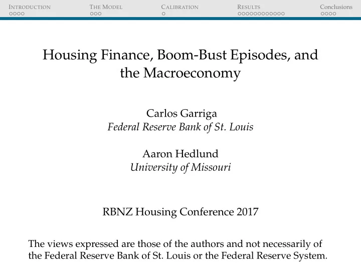
Housing Finance, Boom-Bust Episodes, and the Macroeconomy Carlos - PowerPoint PPT Presentation
I NTRODUCTION T HE M ODEL C ALIBRATION R ESULTS Conclusions Housing Finance, Boom-Bust Episodes, and the Macroeconomy Carlos Garriga Federal Reserve Bank of St. Louis Aaron Hedlund University of Missouri RBNZ Housing Conference 2017 The
I NTRODUCTION T HE M ODEL C ALIBRATION R ESULTS Conclusions Housing Finance, Boom-Bust Episodes, and the Macroeconomy Carlos Garriga Federal Reserve Bank of St. Louis Aaron Hedlund University of Missouri RBNZ Housing Conference 2017 The views expressed are those of the authors and not necessarily of the Federal Reserve Bank of St. Louis or the Federal Reserve System.
I NTRODUCTION T HE M ODEL C ALIBRATION R ESULTS Conclusions M OTIVATION ◮ According to IMF data, house prices have been soaring globally since the late 90s until the global financial crisis (GFC). ◮ After the GFC prices have continued to grow at a fast pace (i.e. two digit growth in 2017 for countries such as Canada, China, New Zealand, Hong Kong, and single digit U.S. India, Norway) ◮ These global housing booms share common features. ◮ Extended period of credit expansions, lower mortgage borrowing costs alongside a low return to safe assets. ◮ House prices are not driven by rent growth. ◮ House prices are growing more than income.
I NTRODUCTION T HE M ODEL C ALIBRATION R ESULTS Conclusions H OUSING M ARKETS AND C REDIT IN THE U.S. ◮ During the Great Depression, the housing market collapsed as homeowners could not rollover their short-term low LTV loans due to the failure of local banks. ◮ The introduction of high LTV long-term mortgages and nationwide credit were important drivers of the postwar housing boom (Chambers, Garriga, and Schlagenhauf 2012). ◮ 2000s boom was fueled by a credit expansion and declining cost of borrowing. 1.5 2 4 6 3 Real 30-Year FRM Rate 1.4 1.8 Real Mortgage Debt Real Risk-Free Rate 5 Real House Prices 2 1.3 1.6 4 1 1.2 1.4 3 0 1.1 1.2 2 -1 1 1 -2 1 2000 2005 2010 2015 2000 2005 2010 2015 2000 2005 2010 2015 2000 2005 2010 2015
I NTRODUCTION T HE M ODEL C ALIBRATION R ESULTS Conclusions Q UESTIONS AND M ETHODOLOGY Question: How do credit and mortgage arrangements impact the dynamics of housing and the macroeconomy? ◮ Construct a quantitative macro model with extensive and intensive margins for housing and mortgage borrowing. ◮ Analyze the role of credit vs. income-productivity applied to the 2000s housing boom-bust. ◮ Assess the aggregate and cross-sectional implications of mortgage structure. ◮ Evaluate the impact of macroprudential policies targeted at mortgage design.
I NTRODUCTION T HE M ODEL C ALIBRATION R ESULTS Conclusions T AKEAWAYS ◮ Anatomy of the boom: credit booms have a bigger impact on housing and consumption than does income growth. ◮ Asymmetric macro effects: consumption responds more strongly to house price movements during the bust than during the boom. ◮ Mortgage Structure ◮ Refinancing and Equity Extraction: the ability to refinance and extract equity substantially magnifies housing booms and the spillovers to consumption. ◮ Mortgage Duration: long-term debt mitigates rollover risk and has a substantial impact on foreclosure, ownership, and consumption dynamics. ◮ Macroprudential Regulations: Tighter LTV constraints blunt the boom and mitigate the bust. PTI constraints are not as effective at reducing endogenous fragility, but they increase homeownership during the boom.
I NTRODUCTION T HE M ODEL C ALIBRATION R ESULTS Conclusions M ODEL S UMMARY Households � ∞ t = 0 β t u ( c t , c h , t ) . Own h ∈ H with c h = h or ◮ Preferences E 0 consume apartment space c h = a ∈ [ 0 , a ] , a ≤ h . Labor efficiency e · s with cdf F ( e ) and transitions π s ( s ′ | s ) . Technology ◮ Consumption Y c = z c N c . New housing Y h = F h ( L , S h , N h ) . Apartments produced using linear, reversible technology. Long-Term, Defaultable Mortgage Debt ◮ Extensive vs. intensive margins of credit. FRMs vs. ARMs. ◮ Long-term contracts with default, prepayment, and the ability to extract equity. Decentralized Housing Market ◮ Search frictions endogenize housing illiquidity.
I NTRODUCTION T HE M ODEL C ALIBRATION R ESULTS Conclusions H OUSEHOLD P ORTFOLIO C HOICE New buyers/homeowners who refinance: V R ( W own + R sell )( y ′ , ( r m , m ′ ) , h , s ′ , 0 ) � � own ( y , ( r m , m ) , h , s , 0 ) = m ′ , b ′ , c ≥ 0 u ( c , h ) + β E max subject to c + γ p ( h ) + q b b ′ + m ≤ y + q 0 m (( r m , m ′ ) , b ′ , h , s ) m ′ m (( r m , m ′ ) , b ′ , h , s ) m ′ ≤ ϑ p ( h ) q 0 y ′ = we ′ s ′ + b ′ Homeowners who make a regular payment: V C ( W own + R sell )( y ′ , ( r m , m ′ ) , h , s ′ , 0 ) own ( y , ( r m , m ) , h , s , 0 ) = max l , b ′ , c ≥ 0 u ( c , h ) + β E � � subject to c + γ p ( h ) + q b b ′ + l ≤ y r m l ≥ m 1 + r m m ′ = ( m − l )( 1 + r m ) y ′ = we ′ s ′ + b ′
I NTRODUCTION T HE M ODEL C ALIBRATION R ESULTS Conclusions M ORTGAGE F INANCING ◮ Key features: endogenous default premia, prepayment, equity extraction through costly refinancing. ◮ For ARMs, r m = r m adjusts every period. ◮ Mortgage prices satisfy the recursive relationship: sell + repay no sale (do not try/fail) � �� � � �� � 1 m (( r m , m ′ ) , b ′ , h , s ) m ′ = s , h )) m ′ + q 0 η s ( θ s ( p ′ [ 1 − η s ( θ s ( p ′ E s , h ))] ( 1 + ζ )( 1 + r m ) � J REO ( h ) , m ′ � ( 1 + ζ ) q 0 d ′ m (( r m , m ′ ) , b ′′ , h , s ′ ) m ′ × ϕ min + ( 1 − ϕ ) � �� � � �� � � �� � no repossession continuation value with m ′ default + repossession ( 1 + ζ ) q 0 +( 1 − d ′ ) m ′ 1 [ Refi ] + 1 [ No Refi ] m (( r m , m ′′ ) , b ′′ , h , s ′ ) m ′′ l + ���� � �� � payment continuation with m ′′ = ( m ′ − l )( 1 + rm )
I NTRODUCTION T HE M ODEL C ALIBRATION R ESULTS Conclusions C ALIBRATION ◮ Calibrate the economy to the late 1990s. ◮ Important to match the LTV distribution (especially the right tail), homeownership rate, and foreclosures. Description Parameter Value Target Model Source/Reason Homeownership Rate a 2.005 67.0% 67.2% Census Housing Wealth (Owners) ω 0.8177 2.49 2.49 1998 SCF Median Borrower LTV 62.90% 65.51% 1998 SCF Borrowers with LTV ≥ 70 % 40.00% 43.43% 1998 SCF Borrowers with LTV ≥ 80 % β 0.9657 25.0% 24.2% 1998 SCF Borrowers with LTV ≥ 90 % 14.50% 11.27% 1998 SCF Borrowers with LTV ≥ 95 % 9.20% 7.97% 1998 SCF Median Owner Liq. Assets/Earn 0.16 0.15 1998 SCF Foreclosure Starts (Annual) γ s 0.6550 1.60% 1.87% Nat’l Delinquency Survey Full Calibration Details
I NTRODUCTION T HE M ODEL C ALIBRATION R ESULTS Conclusions A NATOMY OF THE H OUSING B OOM 1.5 69 1.5 Credit + Productivity Credit + Productivity Credit + Productivity Productivity Only Productivity Only Productivity Only 1.4 68 1.4 Ownership Rate (%) House Prices Consumption 1.3 67 1.3 1.2 66 1.2 1.1 65 1.1 1 64 1 0 1 2 3 4 5 0 1 2 3 4 5 0 1 2 3 4 5 Time (years) Time (years) Time (years) ◮ Credit booms are much larger than productivity booms. ◮ Consumption increases much more during a credit boom, partly because of housing as an ATM. ◮ The credit boom has a minimal impact on the ownership rate because of the equilibrium increase in house prices.
I NTRODUCTION T HE M ODEL C ALIBRATION R ESULTS Conclusions C REDIT AND THE “N EW N ARRATIVE ” Low Income Middle Income High Income Average Borrower LTV Pre-Boom 59.3% 61.3% 70.3% Productivity Only 56.4% 58.9% 57.1% Productivity + Credit 60.9% 65.8% 69.3% ∆ Credit + 4 . 5 % + 6 . 9 % + 12 . 2 % High-LTV Share ∗ Pre-Boom 13.9% 14.6% 36.3% Productivity + Credit 16.7% 22.7% 31.1% Consumption Change Productivity Only 4.8% 4.2% 1.3% Productivity + Credit 6.0% 11.7% 13.3% ∆ Credit + 1 . 2 % + 7 . 5 % + 12 . 0 % ◮ Broad-based increase in borrowing and consumption from the credit expansion. ◮ Ownership shifts toward larger houses (13% move up with productivity alone vs. 22% when credit also expands).
I NTRODUCTION T HE M ODEL C ALIBRATION R ESULTS Conclusions T HE B OOM , B UST , AND R ECOVERY 50 0.04 Average Time on Market Annual Foreclosure Rate 1.4 40 0.03 House Prices 1.3 1.2 30 0.02 1.1 20 0.01 1 0.9 10 0 0 2 4 6 8 10 0 2 4 6 8 10 0 2 4 6 8 10 Time (years) Time (years) Time (years) Median Borrower Leverage 0.68 1 1.1 Ownership Rate 0.9 0.67 Consumption 1.05 0.8 1 0.66 0.7 0.95 0.65 0.6 0.9 0.64 0.5 0 2 4 6 8 10 0 2 4 6 8 10 0 2 4 6 8 10 Time (years) Time (years) Time (years) ∆ Prices boom ∆ C boom Own boom ∆ Prices bust ∆ C bust Own bust + 44.6% + 12.2% Model 68.1% − 24.5% − 18.5% 64.3% Data + 41.9% + 5.1% 69.2% − 25.9% − 15.0% 64.2% ◮ Downside labor market uncertainty and tighter credit are key to generating the bust.
Recommend
More recommend
Explore More Topics
Stay informed with curated content and fresh updates.

