High-speed cryptography, Speed-oriented Jacobian standards part 2: - PowerPoint PPT Presentation
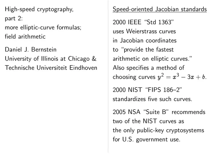
High-speed cryptography, Speed-oriented Jacobian standards part 2: 2000 IEEE Std 1363 more elliptic-curve formulas; uses Weierstrass curves field arithmetic in Jacobian coordinates Daniel J. Bernstein to provide the fastest
Montgomery curves Represent ( ①❀ ② ) as ( ❳ : ❩ ) satisfying ① = ❳❂❩ Chudnovsky–Chudnovsky: 1987 Montgomery: ❇ = ( ❳ 2 + ❩ 2 ) 2 , switching from Use ❜② 2 = ① 3 + ❛① 2 + ① . ❈ = ( ❳ 2 � ❩ 2 ) 2 , ❳❂❩ ❀ ❨❂❩ ❳❂❩❀ ❨❂❩ ). Choose small ( ❛ + 2) ❂ 4. ❛ � 3. ❉ = ❇ � ❈ , ❳ 4 = ❇ ✁ ❈ , ❩ 4 = ❉ ✁ ( ❈ + ❉ ( ❛ + 2) ❂ 4) ✮ 2( ① 2 ❀ ② 2 ) = ( ① 4 ❀ ② 4 ) 2( ❳ 2 : ❩ 2 ) = ( ❳ 4 : ❩ 4 ). ( ① 2 2 � 1) 2 ✮ ① 4 = 2 + ❛① 2 + 1). 4 ① 2 ( ① 2 ignored: ( ❳ 3 : ❩ 3 ) � ( ❳ 2 : ❩ 2 ) = ( ❳ 1 : ❩ etc. ❊ = ( ❳ 3 � ❩ 3 ) ✁ ( ❳ 2 + ❩ 2 ), ( ① 3 ❀ ② 3 ) � ( ① 2 ❀ ② 2 ) = ( ① 1 ❀ ② 1 ), ❋ = ( ❳ 3 + ❩ 3 ) ✁ ( ❳ 2 � ❩ 2 ), ( ① 3 ❀ ② 3 ) + ( ① 2 ❀ ② 2 ) = ( ① 5 ❀ ② 5 ) ❳ 5 = ❩ 1 ✁ ( ❊ + ❋ ) 2 , ✮ ① 5 = ( ① 2 ① 3 � 1) 2 ❩ 5 = ❳ 1 ✁ ( ❊ � ❋ ) 2 ✮ verification. ① 1 ( ① 2 � ① 3 ) 2 . ( ❳ 3 : ❩ 3 ) + ( ❳ 2 : ❩ 2 ) = ( ❳ 5 : ❩
Montgomery curves Represent ( ①❀ ② ) as ( ❳ : ❩ ) satisfying ① = ❳❂❩ . 1987 Montgomery: ❇ = ( ❳ 2 + ❩ 2 ) 2 , Use ❜② 2 = ① 3 + ❛① 2 + ① . ❈ = ( ❳ 2 � ❩ 2 ) 2 , Choose small ( ❛ + 2) ❂ 4. ❉ = ❇ � ❈ , ❳ 4 = ❇ ✁ ❈ , ❩ 4 = ❉ ✁ ( ❈ + ❉ ( ❛ + 2) ❂ 4) ✮ 2( ① 2 ❀ ② 2 ) = ( ① 4 ❀ ② 4 ) 2( ❳ 2 : ❩ 2 ) = ( ❳ 4 : ❩ 4 ). ( ① 2 2 � 1) 2 ✮ ① 4 = 2 + ❛① 2 + 1). 4 ① 2 ( ① 2 ( ❳ 3 : ❩ 3 ) � ( ❳ 2 : ❩ 2 ) = ( ❳ 1 : ❩ 1 ), ❊ = ( ❳ 3 � ❩ 3 ) ✁ ( ❳ 2 + ❩ 2 ), ( ① 3 ❀ ② 3 ) � ( ① 2 ❀ ② 2 ) = ( ① 1 ❀ ② 1 ), ❋ = ( ❳ 3 + ❩ 3 ) ✁ ( ❳ 2 � ❩ 2 ), ( ① 3 ❀ ② 3 ) + ( ① 2 ❀ ② 2 ) = ( ① 5 ❀ ② 5 ) ❳ 5 = ❩ 1 ✁ ( ❊ + ❋ ) 2 , ✮ ① 5 = ( ① 2 ① 3 � 1) 2 ❩ 5 = ❳ 1 ✁ ( ❊ � ❋ ) 2 ✮ ① 1 ( ① 2 � ① 3 ) 2 . ( ❳ 3 : ❩ 3 ) + ( ❳ 2 : ❩ 2 ) = ( ❳ 5 : ❩ 5 ).
Montgomery curves Represent ( ①❀ ② ) This repre as ( ❳ : ❩ ) satisfying ① = ❳❂❩ . does not Montgomery: DADD, “differential ❇ = ( ❳ 2 + ❩ 2 ) 2 , ❜② 2 = ① 3 + ❛① 2 + ① . ◗❀ ❘❀ ◗ � ❘ ✼✦ ◗ ❘ ❈ = ( ❳ 2 � ❩ 2 ) 2 , ose small ( ❛ + 2) ❂ 4. ❉ = ❇ � ❈ , ❳ 4 = ❇ ✁ ❈ , e.g. 2 P❀ P❀ P ✼✦ P ❩ 4 = ❉ ✁ ( ❈ + ❉ ( ❛ + 2) ❂ 4) ✮ e.g. 3 P❀ P❀ P ✼✦ P ① ❀ ② 2 ) = ( ① 4 ❀ ② 4 ) 2( ❳ 2 : ❩ 2 ) = ( ❳ 4 : ❩ 4 ). e.g. 6 P❀ P❀ P ✼✦ P ( ① 2 2 � 1) 2 ✮ ① = 2 + ❛① 2 + 1). 4 ① 2 ( ① 2 ( ❳ 3 : ❩ 3 ) � ( ❳ 2 : ❩ 2 ) = ( ❳ 1 : ❩ 1 ), 2 M + 2 S ❊ = ( ❳ 3 � ❩ 3 ) ✁ ( ❳ 2 + ❩ 2 ), 4 M + 2 S ① ❀ ② ) � ( ① 2 ❀ ② 2 ) = ( ① 1 ❀ ② 1 ), ❋ = ( ❳ 3 + ❩ 3 ) ✁ ( ❳ 2 � ❩ 2 ), Save 1 M ❩ ① ❀ ② ) + ( ① 2 ❀ ② 2 ) = ( ① 5 ❀ ② 5 ) ❳ 5 = ❩ 1 ✁ ( ❊ + ❋ ) 2 , Easily compute ♥ ❳ ❩ ✮ ① = ( ① 2 ① 3 � 1) 2 ❩ 5 = ❳ 1 ✁ ( ❊ � ❋ ) 2 ✮ ① 1 ( ① 2 � ① 3 ) 2 . ✙ lg ♥ DBL, ✙ ♥ ( ❳ 3 : ❩ 3 ) + ( ❳ 2 : ❩ 2 ) = ( ❳ 5 : ❩ 5 ). Almost as ♥P Relatively ♠P ♥◗
curves Represent ( ①❀ ② ) This representation as ( ❳ : ❩ ) satisfying ① = ❳❂❩ . does not allow ADD Montgomery: DADD, “differential ❇ = ( ❳ 2 + ❩ 2 ) 2 , ❛① 2 + ① . ❜② ① ◗❀ ❘❀ ◗ � ❘ ✼✦ ◗ + ❘ ❈ = ( ❳ 2 � ❩ 2 ) 2 , ❛ + 2) ❂ 4. ❉ = ❇ � ❈ , ❳ 4 = ❇ ✁ ❈ , e.g. 2 P❀ P❀ P ✼✦ 3 P ❩ 4 = ❉ ✁ ( ❈ + ❉ ( ❛ + 2) ❂ 4) ✮ e.g. 3 P❀ 2 P❀ P ✼✦ 5 P ① ❀ ② ① ❀ ② 4 ) 2( ❳ 2 : ❩ 2 ) = ( ❳ 4 : ❩ 4 ). e.g. 6 P❀ 5 P❀ P ✼✦ 11 P ① � 1) 2 ✮ ① ① + ❛① 2 + 1). ( ❳ 3 : ❩ 3 ) � ( ❳ 2 : ❩ 2 ) = ( ❳ 1 : ❩ 1 ), 2 M + 2 S + 1 D for ① ❊ = ( ❳ 3 � ❩ 3 ) ✁ ( ❳ 2 + ❩ 2 ), 4 M + 2 S for DADD. � ① ❀ ② 2 ) = ( ① 1 ❀ ② 1 ), ① ❀ ② ❋ = ( ❳ 3 + ❩ 3 ) ✁ ( ❳ 2 � ❩ 2 ), Save 1 M if ❩ 1 = 1. ① ❀ ② ① ❀ ② 2 ) = ( ① 5 ❀ ② 5 ) ❳ 5 = ❩ 1 ✁ ( ❊ + ❋ ) 2 , Easily compute ♥ ( ❳ ❩ ① ① � 1) 2 ❩ 5 = ❳ 1 ✁ ( ❊ � ❋ ) 2 ✮ ✮ ① ① � ① 3 ) 2 . ✙ lg ♥ DBL, ✙ lg ♥ ① ( ❳ 3 : ❩ 3 ) + ( ❳ 2 : ❩ 2 ) = ( ❳ 5 : ❩ 5 ). Almost as fast as Edw ♥P Relatively slow for ♠P ♥◗
Represent ( ①❀ ② ) This representation as ( ❳ : ❩ ) satisfying ① = ❳❂❩ . does not allow ADD but it allo DADD, “differential addition”: ❇ = ( ❳ 2 + ❩ 2 ) 2 , ❜② ① ❛① ① ◗❀ ❘❀ ◗ � ❘ ✼✦ ◗ + ❘ . ❈ = ( ❳ 2 � ❩ 2 ) 2 , ❛ ❂ ❉ = ❇ � ❈ , ❳ 4 = ❇ ✁ ❈ , e.g. 2 P❀ P❀ P ✼✦ 3 P . ❩ 4 = ❉ ✁ ( ❈ + ❉ ( ❛ + 2) ❂ 4) ✮ e.g. 3 P❀ 2 P❀ P ✼✦ 5 P . ① ❀ ② ① ❀ ② 2( ❳ 2 : ❩ 2 ) = ( ❳ 4 : ❩ 4 ). e.g. 6 P❀ 5 P❀ P ✼✦ 11 P . ① � ✮ ① 1). ( ❳ 3 : ❩ 3 ) � ( ❳ 2 : ❩ 2 ) = ( ❳ 1 : ❩ 1 ), 2 M + 2 S + 1 D for DBL. ① ① ❛① ❊ = ( ❳ 3 � ❩ 3 ) ✁ ( ❳ 2 + ❩ 2 ), 4 M + 2 S for DADD. ① ❀ ② 1 ), ① ❀ ② � ① ❀ ② ❋ = ( ❳ 3 + ❩ 3 ) ✁ ( ❳ 2 � ❩ 2 ), Save 1 M if ❩ 1 = 1. ① ❀ ② ① ❀ ② ① ❀ ② 5 ) ❳ 5 = ❩ 1 ✁ ( ❊ + ❋ ) 2 , Easily compute ♥ ( ❳ 1 : ❩ 1 ) using ❩ 5 = ❳ 1 ✁ ( ❊ � ❋ ) 2 ✮ ① ① � ✮ ① ✙ lg ♥ DBL, ✙ lg ♥ DADD. ① ① � ① ( ❳ 3 : ❩ 3 ) + ( ❳ 2 : ❩ 2 ) = ( ❳ 5 : ❩ 5 ). Almost as fast as Edwards ♥P Relatively slow for ♠P + ♥◗
Represent ( ①❀ ② ) This representation as ( ❳ : ❩ ) satisfying ① = ❳❂❩ . does not allow ADD but it allows DADD, “differential addition”: ❇ = ( ❳ 2 + ❩ 2 ) 2 , ◗❀ ❘❀ ◗ � ❘ ✼✦ ◗ + ❘ . ❈ = ( ❳ 2 � ❩ 2 ) 2 , ❉ = ❇ � ❈ , ❳ 4 = ❇ ✁ ❈ , e.g. 2 P❀ P❀ P ✼✦ 3 P . ❩ 4 = ❉ ✁ ( ❈ + ❉ ( ❛ + 2) ❂ 4) ✮ e.g. 3 P❀ 2 P❀ P ✼✦ 5 P . 2( ❳ 2 : ❩ 2 ) = ( ❳ 4 : ❩ 4 ). e.g. 6 P❀ 5 P❀ P ✼✦ 11 P . ( ❳ 3 : ❩ 3 ) � ( ❳ 2 : ❩ 2 ) = ( ❳ 1 : ❩ 1 ), 2 M + 2 S + 1 D for DBL. ❊ = ( ❳ 3 � ❩ 3 ) ✁ ( ❳ 2 + ❩ 2 ), 4 M + 2 S for DADD. ❋ = ( ❳ 3 + ❩ 3 ) ✁ ( ❳ 2 � ❩ 2 ), Save 1 M if ❩ 1 = 1. ❳ 5 = ❩ 1 ✁ ( ❊ + ❋ ) 2 , Easily compute ♥ ( ❳ 1 : ❩ 1 ) using ❩ 5 = ❳ 1 ✁ ( ❊ � ❋ ) 2 ✮ ✙ lg ♥ DBL, ✙ lg ♥ DADD. ( ❳ 3 : ❩ 3 ) + ( ❳ 2 : ❩ 2 ) = ( ❳ 5 : ❩ 5 ). Almost as fast as Edwards ♥P . Relatively slow for ♠P + ♥◗ etc.
resent ( ①❀ ② ) This representation Doubling-o ❳ ❩ ) satisfying ① = ❳❂❩ . does not allow ADD but it allows 2006 Do DADD, “differential addition”: ❳ 2 + ❩ 2 ) 2 , ❇ Use ② 2 = ① ❛① ❛① ◗❀ ❘❀ ◗ � ❘ ✼✦ ◗ + ❘ . ❳ 2 � ❩ 2 ) 2 , ❈ Choose small ❛ ❉ ❇ � ❈ , ❳ 4 = ❇ ✁ ❈ , e.g. 2 P❀ P❀ P ✼✦ 3 P . Use ( ❳ : ❨ ❩ ❩ ❩ ❉ ✁ ( ❈ + ❉ ( ❛ + 2) ❂ 4) ✮ e.g. 3 P❀ 2 P❀ P ✼✦ 5 P . to represent ❳❂❩❀ ❨❂❩ ❳ ❩ 2 ) = ( ❳ 4 : ❩ 4 ). e.g. 6 P❀ 5 P❀ P ✼✦ 11 P . 3 M + 4 S ❳ ❩ ) � ( ❳ 2 : ❩ 2 ) = ( ❳ 1 : ❩ 1 ), 2 M + 2 S + 1 D for DBL. How? Facto ✬ ✬ ❊ ❳ 3 � ❩ 3 ) ✁ ( ❳ 2 + ❩ 2 ), 4 M + 2 S for DADD. where ✬ ❋ ❳ 3 + ❩ 3 ) ✁ ( ❳ 2 � ❩ 2 ), Save 1 M if ❩ 1 = 1. ❩ 1 ✁ ( ❊ + ❋ ) 2 , ❳ 2007 Bernstein–Lange: Easily compute ♥ ( ❳ 1 : ❩ 1 ) using ❳ 1 ✁ ( ❊ � ❋ ) 2 ✮ ❩ 2 M + 5 S ✙ lg ♥ DBL, ✙ lg ♥ DADD. ❳ ❩ ) + ( ❳ 2 : ❩ 2 ) = ( ❳ 5 : ❩ 5 ). on the same Almost as fast as Edwards ♥P . Relatively slow for ♠P + ♥◗ etc.
①❀ ② This representation Doubling-oriented ❳ ❩ satisfying ① = ❳❂❩ . does not allow ADD but it allows 2006 Doche–Icart–Kohel: DADD, “differential addition”: ❇ ❳ ❩ , Use ② 2 = ① 3 + ❛① 2 ❛① ◗❀ ❘❀ ◗ � ❘ ✼✦ ◗ + ❘ . ❈ ❳ � ❩ , Choose small ❛ . ❉ ❇ � ❈ ❳ = ❇ ✁ ❈ , e.g. 2 P❀ P❀ P ✼✦ 3 P . Use ( ❳ : ❨ : ❩ : ❩ ❩ ❉ ✁ ❈ ❉ ( ❛ + 2) ❂ 4) ✮ e.g. 3 P❀ 2 P❀ P ✼✦ 5 P . to represent ( ❳❂❩❀ ❨❂❩ ❳ ❩ ❳ : ❩ 4 ). e.g. 6 P❀ 5 P❀ P ✼✦ 11 P . 3 M + 4 S + 2 D for ❳ ❩ � ❳ ❩ 2 ) = ( ❳ 1 : ❩ 1 ), 2 M + 2 S + 1 D for DBL. How? Factor DBL ✬ ✬ ❊ ❳ � ❩ ✁ ( ❳ 2 + ❩ 2 ), 4 M + 2 S for DADD. where ✬ is a 2-isogeny ❋ ❳ ❩ ✁ ( ❳ 2 � ❩ 2 ), Save 1 M if ❩ 1 = 1. ❋ ) 2 , ❳ ❩ ✁ ❊ 2007 Bernstein–Lange: Easily compute ♥ ( ❳ 1 : ❩ 1 ) using ❳ ✁ ❊ � ❋ ) 2 ✮ ❩ 2 M + 5 S + 2 D for ✙ lg ♥ DBL, ✙ lg ♥ DADD. ❳ ❩ ❳ ❩ 2 ) = ( ❳ 5 : ❩ 5 ). on the same curves. Almost as fast as Edwards ♥P . Relatively slow for ♠P + ♥◗ etc.
①❀ ② This representation Doubling-oriented curves ❳ ❩ ① ❳❂❩ . does not allow ADD but it allows 2006 Doche–Icart–Kohel: DADD, “differential addition”: ❇ ❳ ❩ Use ② 2 = ① 3 + ❛① 2 + 16 ❛① . ◗❀ ❘❀ ◗ � ❘ ✼✦ ◗ + ❘ . ❈ ❳ � ❩ Choose small ❛ . ❉ ❇ � ❈ ❳ ❇ ✁ ❈ e.g. 2 P❀ P❀ P ✼✦ 3 P . Use ( ❳ : ❨ : ❩ : ❩ 2 ) ❩ ❉ ✁ ❈ ❉ ❛ ❂ 4) ✮ e.g. 3 P❀ 2 P❀ P ✼✦ 5 P . to represent ( ❳❂❩❀ ❨❂❩ 2 ). ❳ ❩ ❳ ❩ e.g. 6 P❀ 5 P❀ P ✼✦ 11 P . 3 M + 4 S + 2 D for DBL. ❳ ❩ � ❳ ❩ ❳ : ❩ 1 ), 2 M + 2 S + 1 D for DBL. How? Factor DBL as ˆ ✬ ( ✬ ) ❊ ❳ � ❩ ✁ ❳ ❩ ), 4 M + 2 S for DADD. where ✬ is a 2-isogeny. ❋ ❳ ❩ ✁ ❳ � ❩ ), Save 1 M if ❩ 1 = 1. ❳ ❩ ✁ ❊ ❋ 2007 Bernstein–Lange: Easily compute ♥ ( ❳ 1 : ❩ 1 ) using ❩ ❳ ✁ ❊ � ❋ ✮ 2 M + 5 S + 2 D for DBL ✙ lg ♥ DBL, ✙ lg ♥ DADD. ❳ ❩ ❳ ❩ ❳ : ❩ 5 ). on the same curves. Almost as fast as Edwards ♥P . Relatively slow for ♠P + ♥◗ etc.
This representation Doubling-oriented curves does not allow ADD but it allows 2006 Doche–Icart–Kohel: DADD, “differential addition”: Use ② 2 = ① 3 + ❛① 2 + 16 ❛① . ◗❀ ❘❀ ◗ � ❘ ✼✦ ◗ + ❘ . Choose small ❛ . e.g. 2 P❀ P❀ P ✼✦ 3 P . Use ( ❳ : ❨ : ❩ : ❩ 2 ) e.g. 3 P❀ 2 P❀ P ✼✦ 5 P . to represent ( ❳❂❩❀ ❨❂❩ 2 ). e.g. 6 P❀ 5 P❀ P ✼✦ 11 P . 3 M + 4 S + 2 D for DBL. 2 M + 2 S + 1 D for DBL. How? Factor DBL as ˆ ✬ ( ✬ ) 4 M + 2 S for DADD. where ✬ is a 2-isogeny. Save 1 M if ❩ 1 = 1. 2007 Bernstein–Lange: Easily compute ♥ ( ❳ 1 : ❩ 1 ) using 2 M + 5 S + 2 D for DBL ✙ lg ♥ DBL, ✙ lg ♥ DADD. on the same curves. Almost as fast as Edwards ♥P . Relatively slow for ♠P + ♥◗ etc.
representation Doubling-oriented curves 12 M + 5 not allow ADD but it allows Slower ADD 2006 Doche–Icart–Kohel: ADD, “differential addition”: typically Use ② 2 = ① 3 + ❛① 2 + 16 ❛① . ◗❀ ❘❀ ◗ � ❘ ✼✦ ◗ + ❘ . of the very Choose small ❛ . P❀ P❀ P ✼✦ 3 P . But isogenies Use ( ❳ : ❨ : ❩ : ❩ 2 ) P❀ 2 P❀ P ✼✦ 5 P . Example, to represent ( ❳❂❩❀ ❨❂❩ 2 ). P❀ 5 P❀ P ✼✦ 11 P . fast DBL+D genus-2 3 M + 4 S + 2 D for DBL. 2 S + 1 D for DBL. using simila How? Factor DBL as ˆ ✬ ( ✬ ) 2 S for DADD. where ✬ is a 2-isogeny. M if ❩ 1 = 1. Tricky but tripling-o 2007 Bernstein–Lange: compute ♥ ( ❳ 1 : ❩ 1 ) using (see 2006 2 M + 5 S + 2 D for DBL ✙ ♥ DBL, ✙ lg ♥ DADD. double-base ✿ ✿ ✿ on the same curves. Almost as fast as Edwards ♥P . Relatively slow for ♠P + ♥◗ etc.
sentation Doubling-oriented curves 12 M + 5 S + 1 D fo ADD but it allows Slower ADD than 2006 Doche–Icart–Kohel: “differential addition”: typically outweighing Use ② 2 = ① 3 + ❛① 2 + 16 ❛① . ◗❀ ❘❀ ◗ � ❘ ✼✦ ◗ + ❘ . of the very fast DBL. Choose small ❛ . P❀ P❀ P ✼✦ 3 P . But isogenies are useful. Use ( ❳ : ❨ : ❩ : ❩ 2 ) P❀ P❀ P ✼✦ 5 P . Example, 2005 Gaudry: to represent ( ❳❂❩❀ ❨❂❩ 2 ). P❀ P❀ P ✼✦ 11 P . fast DBL+DADD genus-2 hyperelliptic 3 M + 4 S + 2 D for DBL. for DBL. using similar factorization. How? Factor DBL as ˆ ✬ ( ✬ ) ADD. where ✬ is a 2-isogeny. ❩ 1. Tricky but potentially tripling-oriented cur 2007 Bernstein–Lange: ♥ ( ❳ 1 : ❩ 1 ) using (see 2006 Doche–Ica 2 M + 5 S + 2 D for DBL ✙ ♥ ✙ lg ♥ DADD. double-base chains, ✿ ✿ ✿ on the same curves. as Edwards ♥P . for ♠P + ♥◗ etc.
Doubling-oriented curves 12 M + 5 S + 1 D for ADD. it allows Slower ADD than other systems, 2006 Doche–Icart–Kohel: addition”: typically outweighing benefit Use ② 2 = ① 3 + ❛① 2 + 16 ❛① . ◗❀ ❘❀ ◗ � ❘ ✼✦ ◗ ❘ of the very fast DBL. Choose small ❛ . P❀ P❀ P ✼✦ P But isogenies are useful. Use ( ❳ : ❨ : ❩ : ❩ 2 ) P❀ P❀ P ✼✦ P Example, 2005 Gaudry: to represent ( ❳❂❩❀ ❨❂❩ 2 ). P❀ P❀ P ✼✦ P fast DBL+DADD on Jacobians genus-2 hyperelliptic curves, 3 M + 4 S + 2 D for DBL. using similar factorization. How? Factor DBL as ˆ ✬ ( ✬ ) where ✬ is a 2-isogeny. ❩ Tricky but potentially helpful: tripling-oriented curves 2007 Bernstein–Lange: ♥ ❳ ❩ ) using (see 2006 Doche–Icart–Kohel), 2 M + 5 S + 2 D for DBL ✙ ♥ ✙ ♥ ADD. double-base chains, ✿ ✿ ✿ on the same curves. ♥P . ♠P ♥◗ etc.
Doubling-oriented curves 12 M + 5 S + 1 D for ADD. Slower ADD than other systems, 2006 Doche–Icart–Kohel: typically outweighing benefit Use ② 2 = ① 3 + ❛① 2 + 16 ❛① . of the very fast DBL. Choose small ❛ . But isogenies are useful. Use ( ❳ : ❨ : ❩ : ❩ 2 ) Example, 2005 Gaudry: to represent ( ❳❂❩❀ ❨❂❩ 2 ). fast DBL+DADD on Jacobians of genus-2 hyperelliptic curves, 3 M + 4 S + 2 D for DBL. using similar factorization. How? Factor DBL as ˆ ✬ ( ✬ ) where ✬ is a 2-isogeny. Tricky but potentially helpful: tripling-oriented curves 2007 Bernstein–Lange: (see 2006 Doche–Icart–Kohel), 2 M + 5 S + 2 D for DBL double-base chains, ✿ ✿ ✿ on the same curves.
Doubling-oriented curves 12 M + 5 S + 1 D for ADD. Hessian Slower ADD than other systems, Doche–Icart–Kohel: Credited typically outweighing benefit by 1986 ② = ① 3 + ❛① 2 + 16 ❛① . of the very fast DBL. ose small ❛ . ( ❳ : ❨ : ❩ ❳❂❩❀ ❨❂❩ But isogenies are useful. on ① 3 + ② ❞①② ❳ : ❨ : ❩ : ❩ 2 ) Example, 2005 Gaudry: resent ( ❳❂❩❀ ❨❂❩ 2 ). 12 M for fast DBL+DADD on Jacobians of ❳ 3 = ❨ 1 ❳ ✁ ❨ ❩ � ❩ ❨ ✁ ❳ ❨ genus-2 hyperelliptic curves, 4 S + 2 D for DBL. ❨ 3 = ❳ 1 ❩ ✁ ❳ ❨ � ❨ ❳ ✁ ❩ ❳ using similar factorization. Factor DBL as ˆ ✬ ( ✬ ) ❩ 3 = ❩ 1 ❨ ✁ ❩ ❳ � ❳ ❩ ✁ ❨ ❩ ✬ is a 2-isogeny. Tricky but potentially helpful: 6 M + 3 S tripling-oriented curves Bernstein–Lange: (see 2006 Doche–Icart–Kohel), 5 S + 2 D for DBL double-base chains, ✿ ✿ ✿ same curves.
riented curves 12 M + 5 S + 1 D for ADD. Hessian curves Slower ADD than other systems, rt–Kohel: Credited to Sylvester typically outweighing benefit by 1986 Chudnovsky–Chudnovsky: ❛① 2 + 16 ❛① . ② ① of the very fast DBL. ( ❳ : ❨ : ❩ ) represent ❳❂❩❀ ❨❂❩ ❛ But isogenies are useful. on ① 3 + ② 3 + 1 = ❞①② ❩ 2 ) ❳ ❨ ❩ Example, 2005 Gaudry: ❳❂❩❀ ❨❂❩ 2 ). 12 M for ADD: fast DBL+DADD on Jacobians of ❳ 3 = ❨ 1 ❳ 2 ✁ ❨ 1 ❩ 2 � ❩ ❨ ✁ ❳ ❨ genus-2 hyperelliptic curves, for DBL. ❨ 3 = ❳ 1 ❩ 2 ✁ ❳ 1 ❨ 2 � ❨ ❳ ✁ ❩ ❳ using similar factorization. DBL as ˆ ✬ ( ✬ ) ❩ 3 = ❩ 1 ❨ 2 ✁ ❩ 1 ❳ 2 � ❳ ❩ ✁ ❨ ❩ ✬ 2-isogeny. Tricky but potentially helpful: 6 M + 3 S for DBL. tripling-oriented curves Bernstein–Lange: (see 2006 Doche–Icart–Kohel), for DBL double-base chains, ✿ ✿ ✿ curves.
12 M + 5 S + 1 D for ADD. Hessian curves Slower ADD than other systems, Credited to Sylvester typically outweighing benefit by 1986 Chudnovsky–Chudnovsky: ② ① ❛① ❛① . of the very fast DBL. ( ❳ : ❨ : ❩ ) represent ( ❳❂❩❀ ❨❂❩ ❛ But isogenies are useful. on ① 3 + ② 3 + 1 = 3 ❞①② . ❳ ❨ ❩ ❩ Example, 2005 Gaudry: ❳❂❩❀ ❨❂❩ 12 M for ADD: fast DBL+DADD on Jacobians of ❳ 3 = ❨ 1 ❳ 2 ✁ ❨ 1 ❩ 2 � ❩ 1 ❨ 2 ✁ ❳ ❨ genus-2 hyperelliptic curves, ❨ 3 = ❳ 1 ❩ 2 ✁ ❳ 1 ❨ 2 � ❨ 1 ❳ 2 ✁ ❩ ❳ using similar factorization. ✬ ✬ ) ❩ 3 = ❩ 1 ❨ 2 ✁ ❩ 1 ❳ 2 � ❳ 1 ❩ 2 ✁ ❨ ❩ ✬ Tricky but potentially helpful: 6 M + 3 S for DBL. tripling-oriented curves (see 2006 Doche–Icart–Kohel), double-base chains, ✿ ✿ ✿
12 M + 5 S + 1 D for ADD. Hessian curves Slower ADD than other systems, Credited to Sylvester typically outweighing benefit by 1986 Chudnovsky–Chudnovsky: of the very fast DBL. ( ❳ : ❨ : ❩ ) represent ( ❳❂❩❀ ❨❂❩ ) But isogenies are useful. on ① 3 + ② 3 + 1 = 3 ❞①② . Example, 2005 Gaudry: 12 M for ADD: fast DBL+DADD on Jacobians of ❳ 3 = ❨ 1 ❳ 2 ✁ ❨ 1 ❩ 2 � ❩ 1 ❨ 2 ✁ ❳ 1 ❨ 2 , genus-2 hyperelliptic curves, ❨ 3 = ❳ 1 ❩ 2 ✁ ❳ 1 ❨ 2 � ❨ 1 ❳ 2 ✁ ❩ 1 ❳ 2 , using similar factorization. ❩ 3 = ❩ 1 ❨ 2 ✁ ❩ 1 ❳ 2 � ❳ 1 ❩ 2 ✁ ❨ 1 ❩ 2 . Tricky but potentially helpful: 6 M + 3 S for DBL. tripling-oriented curves (see 2006 Doche–Icart–Kohel), double-base chains, ✿ ✿ ✿
5 S + 1 D for ADD. Hessian curves 2001 Joy ADD than other systems, 2( ❳ 1 : ❨ 1 ❩ Credited to Sylvester ypically outweighing benefit ( ❩ 1 : ❳ 1 ❨ ❨ ❩ ❳ by 1986 Chudnovsky–Chudnovsky: very fast DBL. so can use ( ❳ : ❨ : ❩ ) represent ( ❳❂❩❀ ❨❂❩ ) isogenies are useful. “Unified on ① 3 + ② 3 + 1 = 3 ❞①② . Example, 2005 Gaudry: helpful against 12 M for ADD: DBL+DADD on Jacobians of But need ❳ 3 = ❨ 1 ❳ 2 ✁ ❨ 1 ❩ 2 � ❩ 1 ❨ 2 ✁ ❳ 1 ❨ 2 , genus-2 hyperelliptic curves, 2009 Bernstein–Kohel–Lange: ❨ 3 = ❳ 1 ❩ 2 ✁ ❳ 1 ❨ 2 � ❨ 1 ❳ 2 ✁ ❩ 1 ❳ 2 , similar factorization. Easily avoid ❩ 3 = ❩ 1 ❨ 2 ✁ ❩ 1 ❳ 2 � ❳ 1 ❩ 2 ✁ ❨ 1 ❩ 2 . but potentially helpful: 2008 Hisil–W 6 M + 3 S for DBL. tripling-oriented curves ( ❳ : ❨ : ❩ ❳ ❨ ❩ 2006 Doche–Icart–Kohel), : 2 ❳❨ ❳❩ ❨ ❩ double-base chains, ✿ ✿ ✿ 6 M + 6 S 3 M + 6 S
for ADD. Hessian curves 2001 Joye–Quisquater: than other systems, 2( ❳ 1 : ❨ 1 : ❩ 1 ) = Credited to Sylvester eighing benefit ( ❩ 1 : ❳ 1 : ❨ 1 ) + ( ❨ ❩ ❳ by 1986 Chudnovsky–Chudnovsky: DBL. so can use ADD to ( ❳ : ❨ : ❩ ) represent ( ❳❂❩❀ ❨❂❩ ) re useful. “Unified addition fo on ① 3 + ② 3 + 1 = 3 ❞①② . Gaudry: helpful against side 12 M for ADD: D on Jacobians of But need to permute ❳ 3 = ❨ 1 ❳ 2 ✁ ❨ 1 ❩ 2 � ❩ 1 ❨ 2 ✁ ❳ 1 ❨ 2 , erelliptic curves, 2009 Bernstein–Kohel–Lange: ❨ 3 = ❳ 1 ❩ 2 ✁ ❳ 1 ❨ 2 � ❨ 1 ❳ 2 ✁ ❩ 1 ❳ 2 , factorization. Easily avoid permutation! ❩ 3 = ❩ 1 ❨ 2 ✁ ❩ 1 ❳ 2 � ❳ 1 ❩ 2 ✁ ❨ 1 ❩ 2 . otentially helpful: 2008 Hisil–Wong–Ca ( ❳ : ❨ : ❩ : ❳ 2 : ❨ 6 M + 3 S for DBL. curves ❩ che–Icart–Kohel), : 2 ❳❨ : 2 ❳❩ ❨ ❩ chains, ✿ ✿ ✿ 6 M + 6 S for ADD. 3 M + 6 S for DBL.
Hessian curves 2001 Joye–Quisquater: systems, 2( ❳ 1 : ❨ 1 : ❩ 1 ) = Credited to Sylvester enefit ( ❩ 1 : ❳ 1 : ❨ 1 ) + ( ❨ 1 : ❩ 1 : ❳ by 1986 Chudnovsky–Chudnovsky: so can use ADD to double. ( ❳ : ❨ : ❩ ) represent ( ❳❂❩❀ ❨❂❩ ) “Unified addition formulas,” on ① 3 + ② 3 + 1 = 3 ❞①② . helpful against side channels. 12 M for ADD: Jacobians of But need to permute inputs. ❳ 3 = ❨ 1 ❳ 2 ✁ ❨ 1 ❩ 2 � ❩ 1 ❨ 2 ✁ ❳ 1 ❨ 2 , s, 2009 Bernstein–Kohel–Lange: ❨ 3 = ❳ 1 ❩ 2 ✁ ❳ 1 ❨ 2 � ❨ 1 ❳ 2 ✁ ❩ 1 ❳ 2 , Easily avoid permutation! ❩ 3 = ❩ 1 ❨ 2 ✁ ❩ 1 ❳ 2 � ❳ 1 ❩ 2 ✁ ❨ 1 ❩ 2 . helpful: 2008 Hisil–Wong–Carter–Dawson: ( ❳ : ❨ : ❩ : ❳ 2 : ❨ 2 : ❩ 2 6 M + 3 S for DBL. rt–Kohel), : 2 ❳❨ : 2 ❳❩ : 2 ❨ ❩ ). ✿ ✿ ✿ 6 M + 6 S for ADD. 3 M + 6 S for DBL.
Hessian curves 2001 Joye–Quisquater: 2( ❳ 1 : ❨ 1 : ❩ 1 ) = Credited to Sylvester ( ❩ 1 : ❳ 1 : ❨ 1 ) + ( ❨ 1 : ❩ 1 : ❳ 1 ) by 1986 Chudnovsky–Chudnovsky: so can use ADD to double. ( ❳ : ❨ : ❩ ) represent ( ❳❂❩❀ ❨❂❩ ) “Unified addition formulas,” on ① 3 + ② 3 + 1 = 3 ❞①② . helpful against side channels. 12 M for ADD: But need to permute inputs. ❳ 3 = ❨ 1 ❳ 2 ✁ ❨ 1 ❩ 2 � ❩ 1 ❨ 2 ✁ ❳ 1 ❨ 2 , 2009 Bernstein–Kohel–Lange: ❨ 3 = ❳ 1 ❩ 2 ✁ ❳ 1 ❨ 2 � ❨ 1 ❳ 2 ✁ ❩ 1 ❳ 2 , Easily avoid permutation! ❩ 3 = ❩ 1 ❨ 2 ✁ ❩ 1 ❳ 2 � ❳ 1 ❩ 2 ✁ ❨ 1 ❩ 2 . 2008 Hisil–Wong–Carter–Dawson: ( ❳ : ❨ : ❩ : ❳ 2 : ❨ 2 : ❩ 2 6 M + 3 S for DBL. : 2 ❳❨ : 2 ❳❩ : 2 ❨ ❩ ). 6 M + 6 S for ADD. 3 M + 6 S for DBL.
Hessian curves 2001 Joye–Quisquater: 2( ❳ 1 : ❨ 1 : ❩ 1 ) = Credited to Sylvester ( ❩ 1 : ❳ 1 : ❨ 1 ) + ( ❨ 1 : ❩ 1 : ❳ 1 ) 1986 Chudnovsky–Chudnovsky: so can use ADD to double. ❨ : ❩ ) represent ( ❳❂❩❀ ❨❂❩ ) ❳ “Unified addition formulas,” ① + ② 3 + 1 = 3 ❞①② . helpful against side channels. for ADD: But need to permute inputs. ❨ 1 ❳ 2 ✁ ❨ 1 ❩ 2 � ❩ 1 ❨ 2 ✁ ❳ 1 ❨ 2 , ❳ 2009 Bernstein–Kohel–Lange: ❨ ❳ 1 ❩ 2 ✁ ❳ 1 ❨ 2 � ❨ 1 ❳ 2 ✁ ❩ 1 ❳ 2 , Easily avoid permutation! ① 3 � ② 3 + ✿ ①② ❩ ❩ 1 ❨ 2 ✁ ❩ 1 ❳ 2 � ❳ 1 ❩ 2 ✁ ❨ 1 ❩ 2 . 2008 Hisil–Wong–Carter–Dawson: ( ❳ : ❨ : ❩ : ❳ 2 : ❨ 2 : ❩ 2 3 S for DBL. : 2 ❳❨ : 2 ❳❩ : 2 ❨ ❩ ). 6 M + 6 S for ADD. 3 M + 6 S for DBL.
2001 Joye–Quisquater: 2( ❳ 1 : ❨ 1 : ❩ 1 ) = Sylvester ( ❩ 1 : ❳ 1 : ❨ 1 ) + ( ❨ 1 : ❩ 1 : ❳ 1 ) Chudnovsky–Chudnovsky: so can use ADD to double. resent ( ❳❂❩❀ ❨❂❩ ) ❳ ❨ ❩ “Unified addition formulas,” ① ② = 3 ❞①② . helpful against side channels. But need to permute inputs. ❨ ❳ ✁ ❨ ❩ 2 � ❩ 1 ❨ 2 ✁ ❳ 1 ❨ 2 , ❳ 2009 Bernstein–Kohel–Lange: ❨ ❳ ❩ ✁ ❳ ❨ 2 � ❨ 1 ❳ 2 ✁ ❩ 1 ❳ 2 , Easily avoid permutation! ① 3 � ② 3 + 1 = 0 ✿ 3 ①② ❩ ❩ ❨ ✁ ❩ ❳ 2 � ❳ 1 ❩ 2 ✁ ❨ 1 ❩ 2 . 2008 Hisil–Wong–Carter–Dawson: ( ❳ : ❨ : ❩ : ❳ 2 : ❨ 2 : ❩ 2 DBL. : 2 ❳❨ : 2 ❳❩ : 2 ❨ ❩ ). 6 M + 6 S for ADD. 3 M + 6 S for DBL.
2001 Joye–Quisquater: 2( ❳ 1 : ❨ 1 : ❩ 1 ) = ( ❩ 1 : ❳ 1 : ❨ 1 ) + ( ❨ 1 : ❩ 1 : ❳ 1 ) Chudnovsky–Chudnovsky: so can use ADD to double. ❳❂❩❀ ❨❂❩ ) ❳ ❨ ❩ “Unified addition formulas,” ① ② ❞①② helpful against side channels. But need to permute inputs. ❨ ❳ ✁ ❨ ❩ � ❩ ❨ ✁ ❳ 1 ❨ 2 , ❳ 2009 Bernstein–Kohel–Lange: ❨ ❳ ❩ ✁ ❳ ❨ � ❨ ❳ ✁ ❩ 1 ❳ 2 , Easily avoid permutation! ① 3 � ② 3 + 1 = 0 ✿ 3 ①② ❩ ❩ ❨ ✁ ❩ ❳ � ❳ ❩ ✁ ❨ 1 ❩ 2 . 2008 Hisil–Wong–Carter–Dawson: ( ❳ : ❨ : ❩ : ❳ 2 : ❨ 2 : ❩ 2 : 2 ❳❨ : 2 ❳❩ : 2 ❨ ❩ ). 6 M + 6 S for ADD. 3 M + 6 S for DBL.
2001 Joye–Quisquater: 2( ❳ 1 : ❨ 1 : ❩ 1 ) = ( ❩ 1 : ❳ 1 : ❨ 1 ) + ( ❨ 1 : ❩ 1 : ❳ 1 ) so can use ADD to double. “Unified addition formulas,” helpful against side channels. But need to permute inputs. 2009 Bernstein–Kohel–Lange: Easily avoid permutation! ① 3 � ② 3 + 1 = 0 ✿ 3 ①② 2008 Hisil–Wong–Carter–Dawson: ( ❳ : ❨ : ❩ : ❳ 2 : ❨ 2 : ❩ 2 : 2 ❳❨ : 2 ❳❩ : 2 ❨ ❩ ). 6 M + 6 S for ADD. 3 M + 6 S for DBL.
Joye–Quisquater: ❳ ❨ 1 : ❩ 1 ) = ❩ ❳ 1 : ❨ 1 ) + ( ❨ 1 : ❩ 1 : ❳ 1 ) use ADD to double. “Unified addition formulas,” helpful against side channels. need to permute inputs. Bernstein–Kohel–Lange: avoid permutation! ① 3 � ② 3 + 1 = 0 ✿ 3 ①② Hisil–Wong–Carter–Dawson: ❨ : ❩ : ❳ 2 : ❨ 2 : ❩ 2 ❳ 2 ❳❨ : 2 ❳❩ : 2 ❨ ❩ ). 6 S for ADD. 6 S for DBL.
e–Quisquater: ❳ ❨ ❩ ❩ ❳ ❨ ( ❨ 1 : ❩ 1 : ❳ 1 ) to double. addition formulas,” side channels. ermute inputs. Bernstein–Kohel–Lange: ermutation! ① 3 � ② 3 + 1 = 0 ✿ 3 ①② ong–Carter–Dawson: : ❨ 2 : ❩ 2 ❳ ❨ ❩ ❳ ❳❩ : 2 ❨ ❩ ). ❳❨ ADD. DBL.
❳ ❨ ❩ ❩ ❳ ❨ ❨ ❩ ❳ 1 ) double. rmulas,” channels. inputs. Bernstein–Kohel–Lange: ① 3 � ② 3 + 1 = 0 ✿ 3 ①② rter–Dawson: ❳ ❨ ❩ ❳ ❨ ❩ ❳❨ ❳❩ ❨ ❩
① 3 � ② 3 + 1 = 0 ✿ 3 ①②
Jacobi intersections 1986 Chudnovsky–Chudnovsky: ( ❙ : ❈ : ❉ ❩ ( ❙❂❩❀ ❈❂❩❀ ❉❂❩ s 2 + ❝ 2 = ❛s ❞ 14 M + 2 “Tremendous of being ① � ② 3 + 1 = 0 ✿ 3 ①② 5 M + 3 S “Perhaps ✿ ✿ ✿ efficient which do coefficients
Jacobi intersections 1986 Chudnovsky–Chudnovsky: ( ❙ : ❈ : ❉ : ❩ ) rep ( ❙❂❩❀ ❈❂❩❀ ❉❂❩ ) on s 2 + ❝ 2 = 1, ❛s 2 + ❞ 14 M + 2 S + 1 D fo “Tremendous advantage” of being strongly unified. ✿ 3 ①② ① � ② 5 M + 3 S for DBL. “Perhaps (?) ✿ ✿ ✿ the efficient duplication which do not depend coefficients of an elliptic
Jacobi intersections 1986 Chudnovsky–Chudnovsky: ( ❙ : ❈ : ❉ : ❩ ) represent ( ❙❂❩❀ ❈❂❩❀ ❉❂❩ ) on s 2 + ❝ 2 = 1, ❛s 2 + ❞ 2 = 1. 14 M + 2 S + 1 D for ADD. “Tremendous advantage” of being strongly unified. ① � ② ✿ ①② 5 M + 3 S for DBL. “Perhaps (?) ✿ ✿ ✿ the most efficient duplication formulas which do not depend on the coefficients of an elliptic curve.”
Jacobi intersections 1986 Chudnovsky–Chudnovsky: ( ❙ : ❈ : ❉ : ❩ ) represent ( ❙❂❩❀ ❈❂❩❀ ❉❂❩ ) on s 2 + ❝ 2 = 1, ❛s 2 + ❞ 2 = 1. 14 M + 2 S + 1 D for ADD. “Tremendous advantage” of being strongly unified. 5 M + 3 S for DBL. “Perhaps (?) ✿ ✿ ✿ the most efficient duplication formulas which do not depend on the coefficients of an elliptic curve.”
Jacobi intersections 2001 Lia 13 M + 2 1986 Chudnovsky–Chudnovsky: 4 M + 3 S ( ❙ : ❈ : ❉ : ❩ ) represent 2007 Bernstein–Lange: ( ❙❂❩❀ ❈❂❩❀ ❉❂❩ ) on 3 M + 4 S s 2 + ❝ 2 = 1, ❛s 2 + ❞ 2 = 1. 2008 Hisil–W 14 M + 2 S + 1 D for ADD. 13 M + 1 “Tremendous advantage” 2 M + 5 S of being strongly unified. Also ( ❙ : ❈ ❉ ❩ ❙❈ ❉❩ 5 M + 3 S for DBL. 11 M + 1 “Perhaps (?) ✿ ✿ ✿ the most 2 M + 5 S efficient duplication formulas which do not depend on the coefficients of an elliptic curve.”
Jacobi intersections 2001 Liardet–Smart: 13 M + 2 S + 1 D fo 1986 Chudnovsky–Chudnovsky: 4 M + 3 S for DBL. ( ❙ : ❈ : ❉ : ❩ ) represent 2007 Bernstein–Lange: ( ❙❂❩❀ ❈❂❩❀ ❉❂❩ ) on 3 M + 4 S for DBL. s 2 + ❝ 2 = 1, ❛s 2 + ❞ 2 = 1. 2008 Hisil–Wong–Ca 14 M + 2 S + 1 D for ADD. 13 M + 1 S + 2 D fo “Tremendous advantage” 2 M + 5 S + 1 D for of being strongly unified. Also ( ❙ : ❈ : ❉ : ❩ ❙❈ ❉❩ 5 M + 3 S for DBL. 11 M + 1 S + 2 D fo “Perhaps (?) ✿ ✿ ✿ the most 2 M + 5 S + 1 D for efficient duplication formulas which do not depend on the coefficients of an elliptic curve.”
Jacobi intersections 2001 Liardet–Smart: 13 M + 2 S + 1 D for ADD. 1986 Chudnovsky–Chudnovsky: 4 M + 3 S for DBL. ( ❙ : ❈ : ❉ : ❩ ) represent 2007 Bernstein–Lange: ( ❙❂❩❀ ❈❂❩❀ ❉❂❩ ) on 3 M + 4 S for DBL. s 2 + ❝ 2 = 1, ❛s 2 + ❞ 2 = 1. 2008 Hisil–Wong–Carter–Dawson: 14 M + 2 S + 1 D for ADD. 13 M + 1 S + 2 D for ADD. “Tremendous advantage” 2 M + 5 S + 1 D for DBL. of being strongly unified. Also ( ❙ : ❈ : ❉ : ❩ : ❙❈ : ❉❩ 5 M + 3 S for DBL. 11 M + 1 S + 2 D for ADD. “Perhaps (?) ✿ ✿ ✿ the most 2 M + 5 S + 1 D for DBL. efficient duplication formulas which do not depend on the coefficients of an elliptic curve.”
Jacobi intersections 2001 Liardet–Smart: 13 M + 2 S + 1 D for ADD. 1986 Chudnovsky–Chudnovsky: 4 M + 3 S for DBL. ( ❙ : ❈ : ❉ : ❩ ) represent 2007 Bernstein–Lange: ( ❙❂❩❀ ❈❂❩❀ ❉❂❩ ) on 3 M + 4 S for DBL. s 2 + ❝ 2 = 1, ❛s 2 + ❞ 2 = 1. 2008 Hisil–Wong–Carter–Dawson: 14 M + 2 S + 1 D for ADD. 13 M + 1 S + 2 D for ADD. “Tremendous advantage” 2 M + 5 S + 1 D for DBL. of being strongly unified. Also ( ❙ : ❈ : ❉ : ❩ : ❙❈ : ❉❩ ): 5 M + 3 S for DBL. 11 M + 1 S + 2 D for ADD. “Perhaps (?) ✿ ✿ ✿ the most 2 M + 5 S + 1 D for DBL. efficient duplication formulas which do not depend on the coefficients of an elliptic curve.”
intersections 2001 Liardet–Smart: Jacobi qua 13 M + 2 S + 1 D for ADD. Chudnovsky–Chudnovsky: ( ❳ : ❨ : ❩ ) ❳❂❩❀ ❨❂❩ 4 M + 3 S for DBL. on ② 2 = ① ❛① ❙ ❈ : ❉ : ❩ ) represent 2007 Bernstein–Lange: ❙❂❩❀ ❈❂❩❀ ❉❂❩ ) on 1986 Chudnovsky–Chudnovsky: 3 M + 4 S for DBL. ❝ = 1, ❛s 2 + ❞ 2 = 1. s 3 M + 6 S 2008 Hisil–Wong–Carter–Dawson: Slow ADD. 2 S + 1 D for ADD. 13 M + 1 S + 2 D for ADD. remendous advantage” 2002 Billet–Jo 2 M + 5 S + 1 D for DBL. eing strongly unified. New choic Also ( ❙ : ❈ : ❉ : ❩ : ❙❈ : ❉❩ ): 10 M + 3 3 S for DBL. 11 M + 1 S + 2 D for ADD. strongly erhaps (?) ✿ ✿ ✿ the most 2 M + 5 S + 1 D for DBL. efficient duplication formulas 2007 Bernstein–Lange: do not depend on the 1 M + 9 S efficients of an elliptic curve.”
intersections 2001 Liardet–Smart: Jacobi quartics 13 M + 2 S + 1 D for ADD. Chudnovsky–Chudnovsky: ( ❳ : ❨ : ❩ ) represent ❳❂❩❀ ❨❂❩ 4 M + 3 S for DBL. on ② 2 = ① 4 + 2 ❛① 2 ❙ ❈ ❉ ❩ represent 2007 Bernstein–Lange: ❙❂❩❀ ❈❂❩❀ ❉❂❩ ) on 1986 Chudnovsky–Chudnovsky: 3 M + 4 S for DBL. ❛s + ❞ 2 = 1. s ❝ 3 M + 6 S + 2 D for 2008 Hisil–Wong–Carter–Dawson: Slow ADD. for ADD. 13 M + 1 S + 2 D for ADD. advantage” 2002 Billet–Joye: 2 M + 5 S + 1 D for DBL. unified. New choice of neutral Also ( ❙ : ❈ : ❉ : ❩ : ❙❈ : ❉❩ ): 10 M + 3 S + 1 D fo DBL. 11 M + 1 S + 2 D for ADD. strongly unified. ✿ ✿ ✿ the most 2 M + 5 S + 1 D for DBL. duplication formulas 2007 Bernstein–Lange: depend on the 1 M + 9 S + 1 D for elliptic curve.”
2001 Liardet–Smart: Jacobi quartics 13 M + 2 S + 1 D for ADD. Chudnovsky–Chudnovsky: ( ❳ : ❨ : ❩ ) represent ( ❳❂❩❀ ❨❂❩ 4 M + 3 S for DBL. on ② 2 = ① 4 + 2 ❛① 2 + 1. ❙ ❈ ❉ ❩ 2007 Bernstein–Lange: 1986 Chudnovsky–Chudnovsky: ❙❂❩❀ ❈❂❩❀ ❉❂❩ 3 M + 4 S for DBL. s ❝ ❛s ❞ 1. 3 M + 6 S + 2 D for DBL. 2008 Hisil–Wong–Carter–Dawson: Slow ADD. 13 M + 1 S + 2 D for ADD. 2002 Billet–Joye: 2 M + 5 S + 1 D for DBL. New choice of neutral element. Also ( ❙ : ❈ : ❉ : ❩ : ❙❈ : ❉❩ ): 10 M + 3 S + 1 D for ADD, 11 M + 1 S + 2 D for ADD. strongly unified. ✿ ✿ ✿ 2 M + 5 S + 1 D for DBL. rmulas 2007 Bernstein–Lange: the 1 M + 9 S + 1 D for DBL. curve.”
2001 Liardet–Smart: Jacobi quartics 13 M + 2 S + 1 D for ADD. ( ❳ : ❨ : ❩ ) represent ( ❳❂❩❀ ❨❂❩ 2 ) 4 M + 3 S for DBL. on ② 2 = ① 4 + 2 ❛① 2 + 1. 2007 Bernstein–Lange: 1986 Chudnovsky–Chudnovsky: 3 M + 4 S for DBL. 3 M + 6 S + 2 D for DBL. 2008 Hisil–Wong–Carter–Dawson: Slow ADD. 13 M + 1 S + 2 D for ADD. 2002 Billet–Joye: 2 M + 5 S + 1 D for DBL. New choice of neutral element. Also ( ❙ : ❈ : ❉ : ❩ : ❙❈ : ❉❩ ): 10 M + 3 S + 1 D for ADD, 11 M + 1 S + 2 D for ADD. strongly unified. 2 M + 5 S + 1 D for DBL. 2007 Bernstein–Lange: 1 M + 9 S + 1 D for DBL.
Liardet–Smart: Jacobi quartics 2007 Hisil–Ca 2 S + 1 D for ADD. 2 M + 6 S ( ❳ : ❨ : ❩ ) represent ( ❳❂❩❀ ❨❂❩ 2 ) 3 S for DBL. on ② 2 = ① 4 + 2 ❛① 2 + 1. 2007 Feng–W Bernstein–Lange: 2 M + 6 S 1986 Chudnovsky–Chudnovsky: 4 S for DBL. 1 M + 7 S 3 M + 6 S + 2 D for DBL. on curves ❛ ❝ Hisil–Wong–Carter–Dawson: Slow ADD. 1 S + 2 D for ADD. More speedups: 2002 Billet–Joye: 5 S + 1 D for DBL. 2007 Hisil–Ca New choice of neutral element. ❙ : ❈ : ❉ : ❩ : ❙❈ : ❉❩ ): 2008 Hisil–W 10 M + 3 S + 1 D for ADD, 1 S + 2 D for ADD. use ( ❳ : ❨ ❩ ❳ ❩ strongly unified. 5 S + 1 D for DBL. or ( ❳ : ❨ ❩ ❳ ❩ ❳❩ 2007 Bernstein–Lange: Can combine 1 M + 9 S + 1 D for DBL. Competitive
art: Jacobi quartics 2007 Hisil–Carter–Da for ADD. 2 M + 6 S + 2 D for ( ❳ : ❨ : ❩ ) represent ( ❳❂❩❀ ❨❂❩ 2 ) DBL. on ② 2 = ① 4 + 2 ❛① 2 + 1. 2007 Feng–Wu: Bernstein–Lange: 2 M + 6 S + 1 D for 1986 Chudnovsky–Chudnovsky: DBL. 1 M + 7 S + 3 D for 3 M + 6 S + 2 D for DBL. on curves chosen with ❛ ❝ ong–Carter–Dawson: Slow ADD. for ADD. More speedups: 2007 2002 Billet–Joye: for DBL. 2007 Hisil–Carter–Da New choice of neutral element. ❙ ❈ ❉ : ❩ : ❙❈ : ❉❩ ): 2008 Hisil–Wong–Ca 10 M + 3 S + 1 D for ADD, for ADD. use ( ❳ : ❨ : ❩ : ❳ ❩ strongly unified. or ( ❳ : ❨ : ❩ : ❳ 2 for DBL. ❩ ❳❩ 2007 Bernstein–Lange: Can combine with 1 M + 9 S + 1 D for DBL. Competitive with Edw
Jacobi quartics 2007 Hisil–Carter–Dawson: 2 M + 6 S + 2 D for DBL. ( ❳ : ❨ : ❩ ) represent ( ❳❂❩❀ ❨❂❩ 2 ) on ② 2 = ① 4 + 2 ❛① 2 + 1. 2007 Feng–Wu: 2 M + 6 S + 1 D for DBL. 1986 Chudnovsky–Chudnovsky: 1 M + 7 S + 3 D for DBL 3 M + 6 S + 2 D for DBL. on curves chosen with ❛ 2 + ❝ rter–Dawson: Slow ADD. More speedups: 2007 Duquesne, 2002 Billet–Joye: 2007 Hisil–Carter–Dawson, New choice of neutral element. ❙ ❈ ❉ ❩ ❙❈ ❉❩ ): 2008 Hisil–Wong–Carter–Dawson: 10 M + 3 S + 1 D for ADD, use ( ❳ : ❨ : ❩ : ❳ 2 : ❩ 2 ) strongly unified. or ( ❳ : ❨ : ❩ : ❳ 2 : ❩ 2 : 2 ❳❩ 2007 Bernstein–Lange: Can combine with Feng–Wu. 1 M + 9 S + 1 D for DBL. Competitive with Edwards!
Jacobi quartics 2007 Hisil–Carter–Dawson: 2 M + 6 S + 2 D for DBL. ( ❳ : ❨ : ❩ ) represent ( ❳❂❩❀ ❨❂❩ 2 ) on ② 2 = ① 4 + 2 ❛① 2 + 1. 2007 Feng–Wu: 2 M + 6 S + 1 D for DBL. 1986 Chudnovsky–Chudnovsky: 1 M + 7 S + 3 D for DBL 3 M + 6 S + 2 D for DBL. on curves chosen with ❛ 2 + ❝ 2 = 1. Slow ADD. More speedups: 2007 Duquesne, 2002 Billet–Joye: 2007 Hisil–Carter–Dawson, New choice of neutral element. 2008 Hisil–Wong–Carter–Dawson: 10 M + 3 S + 1 D for ADD, use ( ❳ : ❨ : ❩ : ❳ 2 : ❩ 2 ) strongly unified. or ( ❳ : ❨ : ❩ : ❳ 2 : ❩ 2 : 2 ❳❩ ). 2007 Bernstein–Lange: Can combine with Feng–Wu. 1 M + 9 S + 1 D for DBL. Competitive with Edwards!
quartics 2007 Hisil–Carter–Dawson: 2 M + 6 S + 2 D for DBL. ❳ ❨ ❩ ) represent ( ❳❂❩❀ ❨❂❩ 2 ) ② = ① 4 + 2 ❛① 2 + 1. 2007 Feng–Wu: 2 M + 6 S + 1 D for DBL. Chudnovsky–Chudnovsky: 1 M + 7 S + 3 D for DBL 6 S + 2 D for DBL. on curves chosen with ❛ 2 + ❝ 2 = 1. ADD. More speedups: 2007 Duquesne, Billet–Joye: 2007 Hisil–Carter–Dawson, choice of neutral element. ① 2 = ② 4 � ✿ ② 2008 Hisil–Wong–Carter–Dawson: 3 S + 1 D for ADD, use ( ❳ : ❨ : ❩ : ❳ 2 : ❩ 2 ) strongly unified. or ( ❳ : ❨ : ❩ : ❳ 2 : ❩ 2 : 2 ❳❩ ). Bernstein–Lange: Can combine with Feng–Wu. 9 S + 1 D for DBL. Competitive with Edwards!
2007 Hisil–Carter–Dawson: 2 M + 6 S + 2 D for DBL. resent ( ❳❂❩❀ ❨❂❩ 2 ) ❳ ❨ ❩ ❛① 2 + 1. ② ① 2007 Feng–Wu: 2 M + 6 S + 1 D for DBL. Chudnovsky–Chudnovsky: 1 M + 7 S + 3 D for DBL for DBL. on curves chosen with ❛ 2 + ❝ 2 = 1. More speedups: 2007 Duquesne, e: 2007 Hisil–Carter–Dawson, neutral element. ① 2 = ② 4 � 1 ✿ 9 ② 2 + 2008 Hisil–Wong–Carter–Dawson: for ADD, use ( ❳ : ❨ : ❩ : ❳ 2 : ❩ 2 ) or ( ❳ : ❨ : ❩ : ❳ 2 : ❩ 2 : 2 ❳❩ ). Bernstein–Lange: Can combine with Feng–Wu. for DBL. Competitive with Edwards!
2007 Hisil–Carter–Dawson: 2 M + 6 S + 2 D for DBL. ❳❂❩❀ ❨❂❩ 2 ) ❳ ❨ ❩ ② ① ❛① 2007 Feng–Wu: 2 M + 6 S + 1 D for DBL. Chudnovsky–Chudnovsky: 1 M + 7 S + 3 D for DBL on curves chosen with ❛ 2 + ❝ 2 = 1. More speedups: 2007 Duquesne, 2007 Hisil–Carter–Dawson, element. ① 2 = ② 4 � 1 ✿ 9 ② 2 + 1 2008 Hisil–Wong–Carter–Dawson: use ( ❳ : ❨ : ❩ : ❳ 2 : ❩ 2 ) or ( ❳ : ❨ : ❩ : ❳ 2 : ❩ 2 : 2 ❳❩ ). Can combine with Feng–Wu. Competitive with Edwards!
2007 Hisil–Carter–Dawson: 2 M + 6 S + 2 D for DBL. 2007 Feng–Wu: 2 M + 6 S + 1 D for DBL. 1 M + 7 S + 3 D for DBL on curves chosen with ❛ 2 + ❝ 2 = 1. More speedups: 2007 Duquesne, 2007 Hisil–Carter–Dawson, ① 2 = ② 4 � 1 ✿ 9 ② 2 + 1 2008 Hisil–Wong–Carter–Dawson: use ( ❳ : ❨ : ❩ : ❳ 2 : ❩ 2 ) or ( ❳ : ❨ : ❩ : ❳ 2 : ❩ 2 : 2 ❳❩ ). Can combine with Feng–Wu. Competitive with Edwards!
Hisil–Carter–Dawson: 6 S + 2 D for DBL. eng–Wu: 6 S + 1 D for DBL. 7 S + 3 D for DBL curves chosen with ❛ 2 + ❝ 2 = 1. speedups: 2007 Duquesne, Hisil–Carter–Dawson, ① 2 = ② 4 � 1 ✿ 9 ② 2 + 1 Hisil–Wong–Carter–Dawson: ❳ : ❨ : ❩ : ❳ 2 : ❩ 2 ) ❳ : ❨ : ❩ : ❳ 2 : ❩ 2 : 2 ❳❩ ). combine with Feng–Wu. etitive with Edwards!
rter–Dawson: for DBL. for DBL. for DBL with ❛ 2 + ❝ 2 = 1. 2007 Duquesne, rter–Dawson, ① 2 = ② 4 � 1 ✿ 9 ② 2 + 1 ong–Carter–Dawson: ❳ 2 : ❩ 2 ) ❳ ❨ ❩ ❳ 2 : ❩ 2 : 2 ❳❩ ). ❳ ❨ ❩ with Feng–Wu. with Edwards!
wson: ❝ 2 = 1. ❛ Duquesne, wson, ① 2 = ② 4 � 1 ✿ 9 ② 2 + 1 rter–Dawson: ❳ ❨ ❩ ❳ ❩ ❳ ❨ ❩ ❳ ❩ ❳❩ ). u. rds!
① 2 = ② 4 � 1 ✿ 9 ② 2 + 1
② 4 � 1 ✿ 9 ② 2 + 1 ①
② � ✿ ② + 1 ①
① ② � ✿ ②
More add Explicit-F hyperelliptic.org/EFD EFD has formulas for ADD in 51 rep on 13 shap Not yet handled generalit (e.g., Hessian ✷ complete (e.g., checking ✶
More addition formulas Explicit-Formulas Database: hyperelliptic.org/EFD EFD has 583 computer-verified formulas and operation for ADD, DBL, etc. in 51 representations on 13 shapes of elliptic Not yet handled by generality of curve (e.g., Hessian order ✷ complete addition (e.g., checking for ✶
More addition formulas Explicit-Formulas Database: hyperelliptic.org/EFD EFD has 583 computer-verified formulas and operation counts for ADD, DBL, etc. in 51 representations on 13 shapes of elliptic curves. Not yet handled by computer: generality of curve shapes (e.g., Hessian order ✷ 3 Z ); complete addition algorithms (e.g., checking for ✶ ).
More addition formulas Explicit-Formulas Database: hyperelliptic.org/EFD EFD has 583 computer-verified formulas and operation counts for ADD, DBL, etc. in 51 representations on 13 shapes of elliptic curves. Not yet handled by computer: generality of curve shapes (e.g., Hessian order ✷ 3 Z ); complete addition algorithms (e.g., checking for ✶ ).
More addition formulas How to multiply Explicit-Formulas Database: Standard with coefficients ❢ ❀ ❀ ✿ ✿ ✿ ❀ ❣ hyperelliptic.org/EFD to represent EFD has 583 computer-verified formulas and operation counts Example for ADD, DBL, etc. 839 = 8 ✁ ✁ ✁ in 51 representations value (at t 8 t 2 + 3 t 1 on 13 shapes of elliptic curves. t Not yet handled by computer: Convenient generality of curve shapes inside computer ❀ ❀ (e.g., Hessian order ✷ 3 Z ); (or 9 ❀ 3 ❀ 8 ❀ ❀ ❀ ❀ ❀ ✿ ✿ ✿ complete addition algorithms “ p[0] = (e.g., checking for ✶ ).
More addition formulas How to multiply big Explicit-Formulas Database: Standard idea: Use with coefficients in ❢ ❀ ❀ ✿ ✿ ✿ ❀ ❣ hyperelliptic.org/EFD to represent integer EFD has 583 computer-verified formulas and operation counts Example of representation: 839 = 8 ✁ 10 2 + 3 ✁ for ADD, DBL, etc. ✁ in 51 representations value (at t = 10) of 8 t 2 + 3 t 1 + 9 t 0 . on 13 shapes of elliptic curves. Not yet handled by computer: Convenient to express generality of curve shapes inside computer as ❀ ❀ (e.g., Hessian order ✷ 3 Z ); (or 9 ❀ 3 ❀ 8 ❀ 0 or 9 ❀ 3 ❀ ❀ ❀ ✿ ✿ ✿ complete addition algorithms “ p[0] = 9; p[1] (e.g., checking for ✶ ).
More addition formulas How to multiply big integers Explicit-Formulas Database: Standard idea: Use polynomial with coefficients in ❢ 0 ❀ 1 ❀ ✿ ✿ ✿ ❀ ❣ hyperelliptic.org/EFD to represent integer in radix EFD has 583 computer-verified formulas and operation counts Example of representation: 839 = 8 ✁ 10 2 + 3 ✁ 10 1 + 9 ✁ 10 for ADD, DBL, etc. in 51 representations value (at t = 10) of polynomial 8 t 2 + 3 t 1 + 9 t 0 . on 13 shapes of elliptic curves. Not yet handled by computer: Convenient to express polynomial generality of curve shapes inside computer as array 9 ❀ 3 ❀ (e.g., Hessian order ✷ 3 Z ); (or 9 ❀ 3 ❀ 8 ❀ 0 or 9 ❀ 3 ❀ 8 ❀ 0 ❀ 0 or ✿ ✿ ✿ complete addition algorithms “ p[0] = 9; p[1] = 3; p[2] (e.g., checking for ✶ ).
More addition formulas How to multiply big integers Explicit-Formulas Database: Standard idea: Use polynomial with coefficients in ❢ 0 ❀ 1 ❀ ✿ ✿ ✿ ❀ 9 ❣ hyperelliptic.org/EFD to represent integer in radix 10. EFD has 583 computer-verified formulas and operation counts Example of representation: 839 = 8 ✁ 10 2 + 3 ✁ 10 1 + 9 ✁ 10 0 = for ADD, DBL, etc. in 51 representations value (at t = 10) of polynomial 8 t 2 + 3 t 1 + 9 t 0 . on 13 shapes of elliptic curves. Not yet handled by computer: Convenient to express polynomial generality of curve shapes inside computer as array 9 ❀ 3 ❀ 8 (e.g., Hessian order ✷ 3 Z ); (or 9 ❀ 3 ❀ 8 ❀ 0 or 9 ❀ 3 ❀ 8 ❀ 0 ❀ 0 or ✿ ✿ ✿ ): complete addition algorithms “ p[0] = 9; p[1] = 3; p[2] = 8 ” (e.g., checking for ✶ ).
addition formulas How to multiply big integers Multiply by multiplyin Explicit-Formulas Database: Standard idea: Use polynomial that repre with coefficients in ❢ 0 ❀ 1 ❀ ✿ ✿ ✿ ❀ 9 ❣ hyperelliptic.org/EFD to represent integer in radix 10. Polynomial has 583 computer-verified involves rmulas and operation counts Example of representation: Have split 839 = 8 ✁ 10 2 + 3 ✁ 10 1 + 9 ✁ 10 0 = ADD, DBL, etc. into many representations value (at t = 10) of polynomial 8 t 2 + 3 t 1 + 9 t 0 . shapes of elliptic curves. Example, (8 t 2 + 3 t t et handled by computer: Convenient to express polynomial 64 t 4 + 48 t t t t generality of curve shapes inside computer as array 9 ❀ 3 ❀ 8 Hessian order ✷ 3 Z ); (or 9 ❀ 3 ❀ 8 ❀ 0 or 9 ❀ 3 ❀ 8 ❀ 0 ❀ 0 or ✿ ✿ ✿ ): complete addition algorithms “ p[0] = 9; p[1] = 3; p[2] = 8 ” checking for ✶ ).
rmulas How to multiply big integers Multiply two integers by multiplying polynomial rmulas Database: Standard idea: Use polynomial that represent the with coefficients in ❢ 0 ❀ 1 ❀ ✿ ✿ ✿ ❀ 9 ❣ hyperelliptic.org/EFD to represent integer in radix 10. Polynomial multiplic computer-verified involves small integer eration counts Example of representation: Have split one big 839 = 8 ✁ 10 2 + 3 ✁ 10 1 + 9 ✁ 10 0 = etc. into many small op resentations value (at t = 10) of polynomial 8 t 2 + 3 t 1 + 9 t 0 . elliptic curves. Example, squaring (8 t 2 + 3 t 1 + 9 t 0 ) 2 by computer: Convenient to express polynomial 64 t 4 + 48 t 3 + 153 t t t curve shapes inside computer as array 9 ❀ 3 ❀ 8 rder ✷ 3 Z ); (or 9 ❀ 3 ❀ 8 ❀ 0 or 9 ❀ 3 ❀ 8 ❀ 0 ❀ 0 or ✿ ✿ ✿ ): addition algorithms “ p[0] = 9; p[1] = 3; p[2] = 8 ” for ✶ ).
How to multiply big integers Multiply two integers by multiplying polynomials Database: Standard idea: Use polynomial that represent the integers. with coefficients in ❢ 0 ❀ 1 ❀ ✿ ✿ ✿ ❀ 9 ❣ to represent integer in radix 10. Polynomial multiplication computer-verified involves small integer coefficients. counts Example of representation: Have split one big multiplication 839 = 8 ✁ 10 2 + 3 ✁ 10 1 + 9 ✁ 10 0 = into many small operations. value (at t = 10) of polynomial 8 t 2 + 3 t 1 + 9 t 0 . curves. Example, squaring 839: (8 t 2 + 3 t 1 + 9 t 0 ) 2 = computer: Convenient to express polynomial 64 t 4 + 48 t 3 + 153 t 2 + 54 t 1 + t inside computer as array 9 ❀ 3 ❀ 8 ✷ ); (or 9 ❀ 3 ❀ 8 ❀ 0 or 9 ❀ 3 ❀ 8 ❀ 0 ❀ 0 or ✿ ✿ ✿ ): rithms “ p[0] = 9; p[1] = 3; p[2] = 8 ” ✶
How to multiply big integers Multiply two integers by multiplying polynomials Standard idea: Use polynomial that represent the integers. with coefficients in ❢ 0 ❀ 1 ❀ ✿ ✿ ✿ ❀ 9 ❣ to represent integer in radix 10. Polynomial multiplication involves small integer coefficients. Example of representation: Have split one big multiplication 839 = 8 ✁ 10 2 + 3 ✁ 10 1 + 9 ✁ 10 0 = into many small operations. value (at t = 10) of polynomial 8 t 2 + 3 t 1 + 9 t 0 . Example, squaring 839: (8 t 2 + 3 t 1 + 9 t 0 ) 2 = Convenient to express polynomial 64 t 4 + 48 t 3 + 153 t 2 + 54 t 1 + 81 t 0 . inside computer as array 9 ❀ 3 ❀ 8 (or 9 ❀ 3 ❀ 8 ❀ 0 or 9 ❀ 3 ❀ 8 ❀ 0 ❀ 0 or ✿ ✿ ✿ ): “ p[0] = 9; p[1] = 3; p[2] = 8 ”
to multiply big integers Multiply two integers Oops, pro by multiplying polynomials usually has ❃ Standard idea: Use polynomial that represent the integers. So “carry” coefficients in ❢ 0 ❀ 1 ❀ ✿ ✿ ✿ ❀ 9 ❣ ❝t ❥ ✦ ❜ ❝❂ ❝ t ❥ t ❥ ❝ resent integer in radix 10. Polynomial multiplication involves small integer coefficients. Example, Example of representation: 64 t 4 + 48 t Have split one big multiplication t t t 8 ✁ 10 2 + 3 ✁ 10 1 + 9 ✁ 10 0 = 64 t 4 + 48 t into many small operations. t t t (at t = 10) of polynomial 64 t 4 + 48 t t t t 3 t 1 + 9 t 0 . t Example, squaring 839: 64 t 4 + 63 t t t t (8 t 2 + 3 t 1 + 9 t 0 ) 2 = 70 t 4 + 3 t Convenient to express polynomial t t t 64 t 4 + 48 t 3 + 153 t 2 + 54 t 1 + 81 t 0 . 7 t 5 + 0 t 4 computer as array 9 ❀ 3 ❀ 8 t t t t ❀ 3 ❀ 8 ❀ 0 or 9 ❀ 3 ❀ 8 ❀ 0 ❀ 0 or ✿ ✿ ✿ ): In other = 9; p[1] = 3; p[2] = 8 ”
big integers Multiply two integers Oops, product polynomial by multiplying polynomials usually has coefficients ❃ Use polynomial that represent the integers. So “carry” extra digits: in ❢ 0 ❀ 1 ❀ ✿ ✿ ✿ ❀ 9 ❣ ❝t ❥ ✦ ❜ ❝❂ 10 ❝ t ❥ +1 t ❥ ❝ integer in radix 10. Polynomial multiplication involves small integer coefficients. Example, squaring resentation: 64 t 4 + 48 t 3 + 153 t Have split one big multiplication t t 3 ✁ 10 1 + 9 ✁ 10 0 = ✁ 64 t 4 + 48 t 3 + 153 t into many small operations. t t t 10) of polynomial 64 t 4 + 48 t 3 + 159 t t t t t t Example, squaring 839: 64 t 4 + 63 t 3 + 9 t 2 + t t (8 t 2 + 3 t 1 + 9 t 0 ) 2 = 70 t 4 + 3 t 3 + 9 t 2 + t express polynomial t 64 t 4 + 48 t 3 + 153 t 2 + 54 t 1 + 81 t 0 . 7 t 5 + 0 t 4 + 3 t 3 + 9 t as array 9 ❀ 3 ❀ 8 t t ❀ ❀ ❀ ❀ 3 ❀ 8 ❀ 0 ❀ 0 or ✿ ✿ ✿ ): In other words, 839 = 3; p[2] = 8 ”
gers Multiply two integers Oops, product polynomial by multiplying polynomials usually has coefficients ❃ 9. olynomial that represent the integers. So “carry” extra digits: ❢ ❀ ❀ ✿ ✿ ✿ ❀ 9 ❣ ❝t ❥ ✦ ❜ ❝❂ 10 ❝ t ❥ +1 + ( ❝ mod t ❥ adix 10. Polynomial multiplication involves small integer coefficients. Example, squaring 839: resentation: 64 t 4 + 48 t 3 + 153 t 2 + 54 t 1 + Have split one big multiplication t ✁ 10 0 = ✁ ✁ 64 t 4 + 48 t 3 + 153 t 2 + 62 t 1 + t into many small operations. t olynomial 64 t 4 + 48 t 3 + 159 t 2 + 2 t 1 + t t t t Example, squaring 839: 64 t 4 + 63 t 3 + 9 t 2 + 2 t 1 + 1 t (8 t 2 + 3 t 1 + 9 t 0 ) 2 = 70 t 4 + 3 t 3 + 9 t 2 + 2 t 1 + 1 t 0 olynomial 64 t 4 + 48 t 3 + 153 t 2 + 54 t 1 + 81 t 0 . 7 t 5 + 0 t 4 + 3 t 3 + 9 t 2 + 2 t 1 + t ❀ 3 ❀ 8 ❀ ❀ ❀ ❀ ❀ ❀ ❀ or ✿ ✿ ✿ ): In other words, 839 2 = 703921 p[2] = 8 ”
Recommend
More recommend
Explore More Topics
Stay informed with curated content and fresh updates.

