High-dimensional data analysis Nicolai Meinshausen Seminar f ur - PowerPoint PPT Presentation
High-dimensional data analysis Nicolai Meinshausen Seminar f ur Statistik, ETH Z urich Van Dantzig Seminar, Delft 31 January 2014 Historical start: Microarray data (Golub et al., 1999) Gene expression levels of more than 3000 genes are
High-dimensional data analysis Nicolai Meinshausen Seminar f¨ ur Statistik, ETH Z¨ urich Van Dantzig Seminar, Delft 31 January 2014
Historical start: Microarray data (Golub et al., 1999) Gene expression levels of more than 3000 genes are measured for n = 72 patients, either suffering from acute lymphoblastic leukemia (“X”, 47 cases) or acute myeloid leukemia (“O”, 25 cases). Obtained from Affymetrix oligonucleotide microarrays.
Gene expression analysis cancer 1000-20000 (sub-)type genes 100-1000 people
Large-scale inference problems sample size predictor variables goal gene hundreds of thousands predict cancer expression people of genes (sub-)type webpage millions to billions of billions of word- predict ads webpages and word-pair click-through frequencies rate credict thousands to billions of thousands to billions detect card transactions information pieces about fraudulent fraud transaction/customer transactions medical thousands of tens of thousands to estimate data people billions of indicators risk of for symptoms/drug-use stroke particle millions of millions of classify type physics particle collisions intensity measurements of particles created Inference “works” if we need just a small fraction of variables to make a prediction (but do not yet know which ones).
High-dimensional data Let Y be a real-valued response in R n (binary for classification), X a n × p -dimensional design and assume a linear model in which Y = X β ∗ + ε + δ, P ( Y = 1) = f ( X β ∗ + δ ) , where f ( x ) = 1 / (1 + exp( − x )) for some (sparse) vector β ∗ ∈ R p , noise ε ∈ R n and model error δ ∈ R n . Regression (or classification) is high-dimensional if p ≫ n .
Basis Pursuit (Chen et al. 99) and Lasso (Tibshirani 96) Let Y be the n -dimensional response vector and X the n × p -dimensional design. Basis Pursuit (Chen et al., 99) ˆ β = argmin � β � 1 such that Y = X β. Lasso: β τ = argmin � β � 1 such that � Y − X β � 2 ≤ τ. ˆ Equivalent to (Tibshirani, 96): β λ = argmin � Y − X β � 2 + λ � β � 1 . ˆ Combines sparsity (some ˆ β -components are 0) and convexity. Many variations exist.
Two important properties: Mixing two equally good solutions always improves the fit (as loss function is convex) Mixing solutions produces another valid solution (as feasible sets are convex)
When does it work? For prediction oracle inequalities in the sense that 2 / n ≤ c log( p ) σ 2 s � X (ˆ β − β ∗ ) � 2 n for some constant c > 0, need Restricted Isometry Property (Candes, 2006) or weaker compatibility condition (Geer, 2008). Slower convergence rates possible with weaker assumptions (Greenstein and Ritov, 2004).
When does it work? For prediction oracle inequalities in the sense that 2 / n ≤ c log( p ) σ 2 s � X (ˆ β − β ∗ ) � 2 n for some constant c > 0, need Restricted Isometry Property (Candes, 2006) or weaker compatibility condition (Geer, 2008). Slower convergence rates possible with weaker assumptions (Greenstein and Ritov, 2004). For correct variable selection in the sense that � � ∃ λ : { k : ˆ β λ k � = 0 } = { k : β ∗ k � = 0 } ≈ 1 , P need strong irrepresentable (Zhao and Yu, 2006) or neighbourhood stability condition (NM and B¨ uhlmann, 2006).
Compatibility condition The usual minimal eigenvalue of the design min {� X β � 2 2 : � β � 2 = 1 } always vanishes for high-dimensional data with p > n .
Compatibility condition The usual minimal eigenvalue of the design min {� X β � 2 2 : � β � 2 = 1 } always vanishes for high-dimensional data with p > n . The φ be the ( L , S )-restricted eigenvalue (Geer, 2007): φ 2 ( L , S ) = min { s � X β � 2 2 : � β S � 1 = 1 and � β S c � 1 ≤ L } , where s = | S | and ( β S ) k = β k 1 { k ∈ S } .
1 If φ ( L , S ) > c > 0 for some L > 1, then we get oracle rates for prediction and convergence of � β ∗ − ˆ β λ � 1 . 2 If φ (1 , S ) > 0 and f = X β ∗ for some β ∗ with � β ∗ � 0 ≤ s , then the following two are identical argmin � β � 0 such that X β = f argmin � β � 1 such that X β = f .
1 If φ ( L , S ) > c > 0 for some L > 1, then we get oracle rates for prediction and convergence of � β ∗ − ˆ β λ � 1 . 2 If φ (1 , S ) > 0 and f = X β ∗ for some β ∗ with � β ∗ � 0 ≤ s , then the following two are identical argmin � β � 0 such that X β = f argmin � β � 1 such that X β = f . The latter equivalence requires otherwise the stronger Restricted Isometry Property which implies that ∃ δ < 1 such that (1 − δ ) � b � 2 2 ≤ � Xb � 2 2 ≤ (1 + δ ) � b � 2 ∀ b with � b � 0 ≤ s : 2 , which can be a useful assumption for random designs X , as in compressed sensing.
Three examples: 1 Compressed sensing 2 Electro-retinography 3 Mind reading
Compressed sensing Images are often sparse after taking a wavelet transformation X : u = Xw , where w ∈ R n : original image as n -dimensional vector X ∈ R n × n : wavelet transformation u ∈ R n : vector with wavelet coefficients
Original wavelet transformation: u = Xw , where The wavelet coefficients u are often sparse in the sense that it has only a few large entries. Keeping just a few of them allows a very good reconstruction of the original image w . u = u 1 {| U | ≥ τ } be the hard-thresholded coefficients (easy to store). Let ˜ w = X − 1 ˜ Then re-construct image as ˜ u .
Conventional way: measure image w with 16 million pixels convert to wavelet coefficients u = Xw throw away most of u by keeping just the largest coefficients Is efficient as long as pixels are cheap.
For situations where pixels are expensive (different wavelengths, MRI) can do compressed sensing: observe only y = Φ u = Φ( Xw ) , where for q ≪ n , matrix Φ ∈ R q × n has iid entries drawn from N (0 , 1). One entry of q -dimensional vector y is thus observed by a random transformation of the original image. Each random mask corresponds to one row of Φ. Reconstruct u by Basis Pursuit: u = argmin � ˜ ˆ u � 1 such that Φ˜ u = y .
Observe y = Φ u = Φ( Xw ) , where for q ≪ n , matrix Φ ∈ R q × n has iid entries drawn from N (0 , 1). Reconstruct wavelet coefficients u by Basis Pursuit: u = argmin � ˜ u � 1 such that Φ˜ ˆ u = y .
Observe y = Φ u = Φ( Xw ) , where for q ≪ n , matrix Φ ∈ R q × n has iid entries drawn from N (0 , 1). Reconstruct wavelet coefficients u by Basis Pursuit: u = argmin � ˜ u � 1 such that Φ˜ ˆ u = y . Matrix Φ satisfies for q ≥ s log( p / s ) with high probability the Random Isometry Property , including the existence of a δ < 1 such that (Candes, 2006) for all s -sparse vectors (1 − δ ) � b � 2 2 ≤ � Φ b � 2 2 ≤ (1 + δ ) � b � 2 2 . Hence, if original wavelet coeffcients are s -sparse, we only need to make of order s log( n / s ) measurements to recover u exactly (with high probability)!
Object Light Lens 1 DMD+ALP Board Lens 2 Photodiode circuit dsp.rice.edu/cs/camera
dsp.rice.edu/cs/camera
Retina Checks (Electroretinography) Can one identify “blind” spots on the retina while measuring only the aggregate electrical signal ? �������������������� �������� ����������� ���������� ������ ������������������������������
Assume there are p retinal areas (corresponding to the blocks in the shown patterns) of which some can be unresponsive. stimulus of overall electrical random black-white retinal areas response patterns Can detect s unresponsive retinal areas with just s log( p / s ) random patterns.
Mind reading Can use Lasso-type inference to infer for a single voxel in the early visual cortex which stimuli lead to neuronal activity using fmri-measurements (Nishimoto et al., 2011 at Gallant Lab, UC Berkeley). Voxel A Show movies and detect which parts of the image a particular voxel of 100k neurons is sensitive to.
Voxel A Voxel B Voxel C CV Learn a Lasso regression that predicts neuronal activity in each separate voxel. Dots indicate large regression coefficients and thus important regions for a voxel.
Allows to forecast brain activity at all voxels, given an image. Voxel A ?
Given only brain activity, can reverse the process and ask which image best explains the neuronal activity (given the learned regressions). ?
Four challenges: Trade-off between statistical and computational efficiency Inhomogeneous data Confidence statements Interactions in high dimensions
Interactions Many datasets are only moderately high-dimensional with raw data Activity of approximately 20k genes in microarray data Presence of about 20k words in texts/websites About 15k different symptoms and 15k different drugs recorded in medical histories (US). Interactions look for effects that are caused by simultaneous presence of two or more variables. are two or more genes active at the same time ? do two words appear close together ? have two drugs been taken simultaneously ?
Recommend
More recommend
Explore More Topics
Stay informed with curated content and fresh updates.
