Heuristic Algorithms for Multiobjective Combinatorial Optimization - PDF document

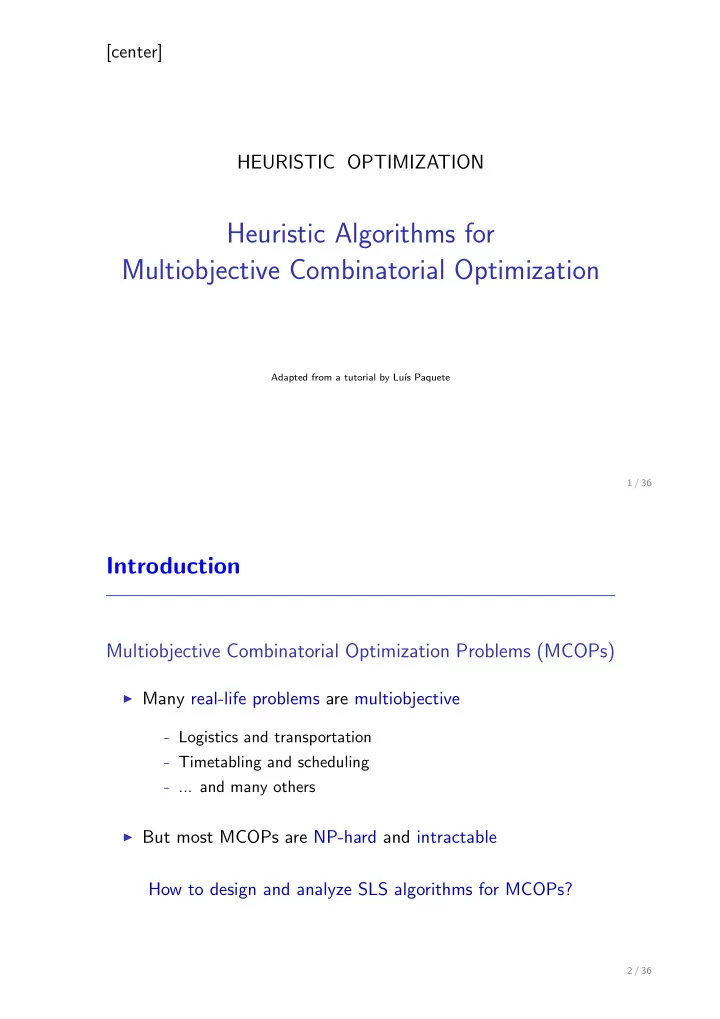
[center] HEURISTIC OPTIMIZATION Heuristic Algorithms for Multiobjective Combinatorial Optimization Adapted from a tutorial by Lu´ ıs Paquete 1 / 36 Introduction Multiobjective Combinatorial Optimization Problems (MCOPs) I Many real-life problems are multiobjective - Logistics and transportation - Timetabling and scheduling - ... and many others I But most MCOPs are NP-hard and intractable How to design and analyze SLS algorithms for MCOPs? 2 / 36

Train roundtrip through capitals of German federal states The fastest roundtrip: I take only ICE trains The cheapest roundtrip: I take only local trains 3 / 36 cost The fastest The cheapest time 4 / 36

cost The fastest The cheapest time 5 / 36 cost The fastest The cheapest time 6 / 36

cost time 7 / 36 cost time 8 / 36

Multiobjective Combinatorial Optimization Problem The set X of feasible solutions is finite and its elements have some combinatorial property (graph, tree, path, partition, etc.). The goal is to min x 2 X f ( x ) = ( f 1 ( x ) , . . . , f Q ( x )) I The objective function f maps x 2 X to R Q 9 / 36 I Optimality depends of the decision maker’s preferences (or lack of them). I Pareto-optimality is based on component-wise order : u  v ( ) u 6 = v and u i  v i , i = 1 , . . . , Q I A solution x 2 X is e ffi cient i ff @ x 0 2 X s.t. f ( x 0 )  f ( x ) I E ffi cient set is the set of all e ffi cient solutions I Nondominated set is the image of the e ffi cient set in f 10 / 36

cost time 11 / 36 MCOPs and Solution Methods I Most MCOPs are NP-hard Decision version of MCOP (MCOP-D) [Serafini 1986]: Given z = ( z 1 , . . . , z Q ), does there exist a solution x 2 X s.t. f ( x )  z or f ( x ) = z ? 1. If the single-objective problem is NP-complete, then the corresponding MCOP-D is also NP-complete. 2. If the single-objective problem is solvable in polynomial time, the corresponding MCOP-D may still be NP-complete. 12 / 36

Solution Methods to MCOPs I Enumeration Methods - Multiobjective Branch & Bound - Multiobjective Dynamic Programming I Scalarized Methods - Solving several related single-objective problems - Weighted Sum, ✏ -constraint, etc. I SLS Algorithms 13 / 36 Weighted Sum Q X I min � i f i ( x ) x 2 X i =1 I � gives a search direction I An optimal solution with � > 0 is e ffi cient. 14 / 36

Weighted Sum Q X I min � i f i ( x ) x 2 X i =1 I � gives a search direction I An optimal solution with � > 0 is e ffi cient. 15 / 36 SLS Algorithms SLS Algorithm design challenges for MCOPs I How to attain more than one solution? I How to attain high quality solutions? I How to evaluate performance? Rule of thumb I Closeness to the nondominated set I Well-distributed outcomes I The more, the better 16 / 36

Scalarized Acceptance Criterion (SAC) Model I Weighted Sum Q X f ( x ) = � i f i ( x ) i =1 I Weighted Chebyche ff � � f ( x ) = max � i | f i ( x ) � y i | i =1 ,..., Q 17 / 36 SAC Search Model cost ————————————– input : weight vectors Λ for each � 2 Λ do x is a candidate solution x 0 = SolveSAC( x , � ) Add x 0 to Archive Filter Archive return Archive ————————————– time 18 / 36

SAC Search Model ———————————— AAA input : weight vectors Λ I Search Strategy for each � 2 Λ do x is a candidate solution I Number of Scalarizations x 0 = SolveSAC( x , � ) I Intensification Mechanism Add x 0 to Archive Filter Archive I Neighborhood return Archive ———————————— 19 / 36 SAC Search Model – EMO ————————————— cost 2 3 input : candidate solution set 1 3 X n 2 3 repeat 2 1 X r = Reproduce/Mutate( X n ) R = Rank( X r , X n ) 2 X s = Select( X r , X n , R ) 1 X n = Replace( X s ) 1 return X n ————————————— time 20 / 36

SAC Search Model – EMO ————————————— cost 3 5 input : candidate solution set 1 5 X n 2 6 repeat 2 1 X r = Reproduce/Mutate( X n ) R = Rank( X r , X n ) 3 X s = Select( X r , X n , R ) 1 X n = Replace( X s ) 1 return X n ————————————— time 21 / 36 SAC Search Model – EMO AA —————————————– input : candidate solution set X n I Component-wise order repeat X r = Reproduce/Mutate( X n ) I Closeness R = Rank( X r , X n ) X s = Select( X r , X n , R ) I Performance indicators X n = Replace( X s ) return X n —————————————– 22 / 36

Multiobjective Local Search ——————————————————————– input :candidate solution x while x is not a local optimum do choose a neighbor x 0 from x such that f ( x 0 )  f ( x ) x = x 0 return x ——————————————————————– I What if f ( x 0 ) and f ( x ) are mutually nondominated? I How to obtain more than a single solution? 23 / 36 CWAC Search Model ———————————— cost input : candidate solution x Add x to Archive repeat Choose x from Archive X N = Neighbors( x ) Add X N to Archive Filter Archive until all x in Archive are visited return Archive ———————————— time 24 / 36

CWAC Search Model ———————————— input : candidate solution x , ✏ Add x to Archive repeat Choose x from Archive X N = Neighbors( x ) Add X N to Archive Filter Archive according to ✏ until all x in Archive are visited return Archive Archive bounding ———————————— [Angel et al. 2004] 25 / 36 Hybrid Search Model ———————————— cost input : weight vectors Λ for each � 2 Λ do x is a candidate solution x 0 = SolveSAC( x , � ) X 0 = CW( x 0 ) Add X 0 to Archive Filter Archive return Archive ———————————— time 26 / 36

Performance Assessment Rules of Thumb: An algorithm performs better if I It is closer to the nondominated set I It has better distributed outcomes I It has more solutions Indicators of Performance I Measure some property of the outcomes I Most of the indicators have limitations [Knowles & Corne 2002, Zitzler et al. 2003] 27 / 36 cost time Many runs of Algorithms Blue and Red 28 / 36

Another example 29 / 36 I Better relations [Hansen & Jaszkiewicz 1998, Zitzler et al. 2003] cost cost time time Blue is better than Red Blue and Red are incomparable 30 / 36

I Unary Indicator: Hypervolume [Zitzler and Thiele, 1998] H ( B ) = 45 H ( W ) = 25 B is better than W = H ( B ) > H ( W ) ) 31 / 36 I Unary Indicator: Hypervolume [Zitzler and Thiele, 1998] H ( B ) = 37 H ( W ) = 36 H ( B ) > H ( W ) = B is not worse than W ) 32 / 36

I Attainment Functions [V.G. da Fonseca et al. 2001] AF : Prob. that an outcome set is better or equal to z . EAF : How many runs an outcome set is better or equal to z ? 33 / 36 I Attainment functions – Visualization of di ff erences EAF Blue � EAF Red positive di ff erences negative di ff erences 34 / 36

I Attainment functions – Statistical testing K-S test statistic: max | EAF Blue � EAF Red | positive di ff erences negative di ff erences 35 / 36 References I Textbooks: R.E. Steuer 1986, K. Miettinen 1999, M. Ehrgott 2005, V.T’kindt et al. 2002, K. Deb 2002. I Reviews: M. Ehrgott and X. Gandibleux 2000, 2002, 2004, 2009, C.C. Coello 2000, D. Jones et al. 2002, J. Knowles and D. Corne 2004, L. Paquete and T. St¨ utzle 2007. I Complexity and Approximation: P. Hansen 1979, P. Serafini 1986, M. Ehrgott 2000, C.H. Papadimitriou and M. Yannakakis 2000, E. Angel et al. 2007. I Performance Assessment: E. Zitzler et al. 2003, 2008, V.G. da Fonseca et al. 2001, 2010, M. Lop´ ez-Ib´ a˜ nez et al. 2010. I Web material: PISA ( http://www.tik.ethz.ch/~sop/pisa ), MOMH ( http://home.gna.org/momh ), ParadisEO ( http://paradiseo.gforge.inria.fr ) 36 / 36