hebma@nju.edu.cn The context of this lecture is based on the - PowerPoint PPT Presentation

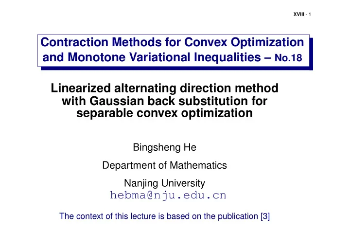
XVIII - 1 Contraction Methods for Convex Optimization and Monotone Variational Inequalities – No.18 Linearized alternating direction method with Gaussian back substitution for separable convex optimization Bingsheng He Department of Mathematics Nanjing University hebma@nju.edu.cn The context of this lecture is based on the publication [3]

XVIII - 2 1 Introduction In this paper, we consider the general case of linearly constrained separable convex programming with m ≥ 3 : � m min i =1 θ i ( x i ) � m i =1 A i x i = b ; (1.1) x i ∈ X i , i = 1 , · · · , m ; where θ i : ℜ n i → ℜ ( i = 1 , . . . , m ) are closed proper convex functions (not necessarily smooth); X i ⊂ ℜ n i ( i = 1 , . . . , m ) are closed convex sets; A i ∈ ℜ l × n i ( i = 1 , . . . , m ) are given matrices and b ∈ ℜ l is a given vector. Throughout, we assume that the solution set of (1.1) is nonempty. In fact, even for the special case of (1.1) with m = 3 , the convergence of the extended ADM is still open. In the last lecture, we provided a novel approach towards the extension of ADM for the problem (1.1). More specifically, we show that if a new iterate is generated by correcting the output of the ADM with a Gaussian back substitution procedure, then the

XVIII - 3 sequence of iterates is convergent to a solution of (1.1). The resulting method is called the ADM with Gaussian back substitution (ADM-GbS). Alternatively, the ADM-GbS can be regarded as a prediction-correction type method whose predictor is generated by the ADM procedure and the correction is completed by a Gaussian back substitution procedure. The main task of each iteration in ADM-GbS is to solve the following sub-problem: 2 � A i x i − b i � 2 | x i ∈ X i } , min { θ i ( x i ) + β i = 1 , . . . , m. (1.2) Thus, ADM-GbS is implementable only when the subproblems of (1.2) have their solutions in the closed form. Again, each iteration of the proposed method in this lecture consists of two steps–prediction and correction. In order to implement the prediction step, we only assume that the x i -subproblem 2 � x i − a i � 2 | x i ∈ X i } , min { θ i ( x i ) + r i i = 1 , . . . , m (1.3) has its solution in the closed form. The first-order optimality condition of (1.1) and thus characterize (1.1) by a variational inequality (VI). As we will show, the VI characterization is convenient for the convergence analysis to be conducted.

XVIII - 4 By attaching a Lagrange multiplier vector λ ∈ ℜ l to the linear constraint, the Lagrange function of (1.1) is: m m θ i ( x i ) − λ T ( � � L ( x 1 , x 2 , . . . , x m , λ ) = A i x i − b ) , (1.4) i =1 i =1 which is defined on W := X 1 × X 2 × · · · × X m × ℜ l . x ∗ 1 , x ∗ 2 , . . . , x ∗ m , λ ∗ � � Let be a saddle point of the Lagrange function (1.4). Then we have L λ ∈ℜ l ( x ∗ 1 , x ∗ 2 , · · · , x ∗ L ( x ∗ 1 , x ∗ 2 , · · · , x ∗ m , λ ∗ ) m , λ ) ≤ L x i ∈X i ( i =1 ,...,m ) ( x 1 , x 2 , . . . , x m , λ ∗ ) . ≤ For i ∈ { 1 , 2 , · · · , m } , we denote by ∂θ i ( x i ) the subdifferential of the convex function θ i ( x i ) and by f i ( x i ) ∈ ∂θ i ( x i ) a given subgradient of θ i ( x i ) . It is evident that finding a saddle point of L ( x 1 , x 2 , . . . , x m , λ ) is equivalent to finding

XVIII - 5 w ∗ = ( x ∗ 1 , x ∗ 2 , ..., x ∗ m , λ ∗ ) ∈ W , such that  1 ) T { f 1 ( x ∗ ( x 1 − x ∗ 1 ) − A T 1 λ ∗ } ≥ 0 ,    .  .   . (1.5) m ) T { f m ( x ∗ ( x m − x ∗ m ) − A T m λ ∗ } ≥ 0 ,    ( λ − λ ∗ ) T ( � m  i =1 A i x ∗  i − b ) ≥ 0 ,  for all w = ( x 1 , x 2 , · · · , x m , λ ) ∈ W . More compactly, (1.5) can be written into ( w − w ∗ ) T F ( w ∗ ) ≥ 0 , ∀ w ∈ W , (1.6a) where     f 1 ( x 1 ) − A T x 1 1 λ . .     . .     . . w = F ( w ) = .   and   (1.6b)    f m ( x m ) − A T  x m m λ         � m λ i =1 A i x i − b Note that the operator F ( w ) defined in (1.6b) is monotone due to the fact that θ i ’s are all convex functions. In addition, the solution set of (1.6), denoted by W ∗ , is also nonempty.

XVIII - 6 2 Linearized ADM with Gaussian back substitution 2.1 Linearized ADM Prediction w k = (˜ m , ˜ x k x k x k λ k ) in the Step 1. ADM step (prediction step) . Obtain ˜ 1 , ˜ 2 , · · · , ˜ forward (alternating) order by the following ADM procedure:  � x 1 ∈ X 1 x k θ 1 ( x 1 )+ q T 1 A 1 x 1 + r 1 2 � x 1 − x k 1 � 2 � � � ˜ 1 =arg min ;    .  .   .    i A i x i + r i i � 2 �  x k θ i ( x i )+ q T 2 � x i − x k � � ˜ i =arg min � x i ∈ X i ;     .  .  . � x m ∈ X m m � 2 � x k � θ m ( x m ) + q T m A m x m + r m 2 � x m − x k � ˜ m =arg min ;       q i = β ( � i − 1 j + � m x k j = i A j x k  j =1 A j ˜ j − b ) . where       λ k = λ k − β ( � m  ˜ x k  j =1 A j ˜ j − b ) .  (2.1)

XVIII - 7 The prediction is implementable due to the assumption (1.3) of this lecture and � � i � 2 � θ i ( x i )+ q T i A i x i + r i 2 � x i − x k arg min � x i ∈ X i � � x k r i A T � 2 � θ i ( x i ) + r i i − 1 � � = arg min 2 � x i − � x i ∈ X i i q i . r i , i = 1 , . . . , m is chosen that condition Assumption i � 2 ≥ β � A i ( x k i ) � 2 r i � x k x k x k i − ˜ i − ˜ (2.2) is satisfied in each iteration. In the case that A i = I n i , we take r i = β , the condition (2.2) is satisfied. Note that in this case we have i − 1 m � � A i x i + β � T � � � i � 2 x k A j x k 2 � x i − x k argmin θ i ( x i )+ β ( A j ˜ j + j − b ) x i ∈X i j =1 j = i � i − 1 m � 2 � − 1 θ i ( x i )+ β � β λ k � � � x k � A j x k = argmin A j ˜ j + A i x i + j − b . � � 2 � � x i ∈X i j =1 j = i +1

XVIII - 8 2.2 Correction by the Gaussian back substitution To present the Gaussian back substitution procedure, we define the matrices:   0 · · · · · · 0 r 1 I n 1     . ...   . βA T  2 A 1 r 2 I n 2  .       . .   ... ... ... M = , (2.3) . .   . .         βA T βA T · · · 0 m A 1 m A m − 1 r m I n m         1 0 0 · · · 0 β I l and r 1 I n 1 , r 2 I n 2 , . . . , r m I n m , 1 � � H = diag β I . (2.4) l Note that for β > 0 and r i > 0 , the matrix M defined in (2.3) is a non-singular

XVIII - 9 lower-triangular block matrix. In addition, according to (2.3) and (2.4), we have:   r 1 A T β r 1 A T β · · · 0 I n 2 1 A 2 1 A m         . . ... ... . .   0 . .           H − 1 M T = .   ... . . r nm − 1 A T β   I n m − 1 m − 1 A m 0 .             0 · · · 0 0 I n m           0 · · · 0 0 I l (2.5) which is a upper-triangular block matrix whose diagonal components are identity matrices. The Gaussian back substitution procedure to be proposed is based on the matrix H − 1 M T defined in (2.5).

XVIII - 10 Step 2. Gaussian back substitution step (correction step) . Correct the ADM output w k in the backward order by the following Gaussian back substitution procedure and ˜ generate the new iterate w k +1 : H − 1 M T ( w k +1 − w k ) = α w k − w k � � ˜ . (2.6) Recall that the matrix H − 1 M T defined in (2.5) is a upper-triangular block matrix. The Gaussian back substitution step (2.6) is thus very easy to execute. In fact, as we mentioned, after the predictor is generated by the linearized ADM scheme (2.1) in the forward (alternating) order, the proposed Gaussian back substitution step corrects the predictor in the backward order. Since the Gaussian back substitution step is easy to perform, the computation of each iteration of the ADM with Gaussian back substitution is dominated by the ADM procedure (2.1). To show the main idea with clearer notation, we restrict our theoretical discussion to the case with fixed β > 0 . The main task of the Gaussian back substitution step (2.6) can be rewritten into w k +1 = w k − αM − T H ( w k − ˜ w k ) . (2.7) As we will show, − M − T H ( w k − ˜ w k ) is a descent direction of the distance function