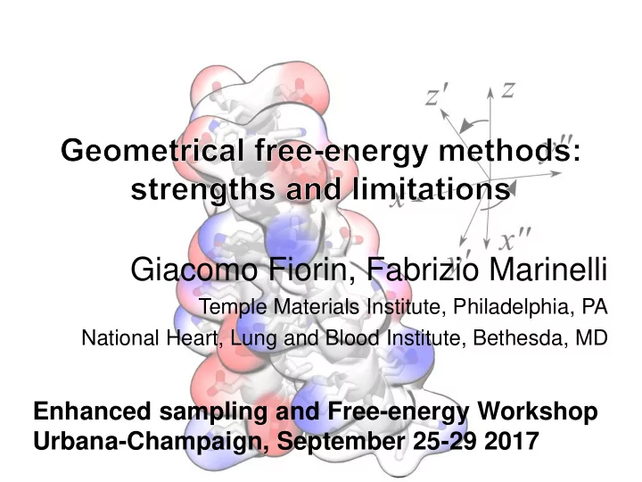
Giacomo Fiorin, Fabrizio Marinelli Temple Materials Institute, - PowerPoint PPT Presentation

Giacomo Fiorin, Fabrizio Marinelli Temple Materials Institute, Philadelphia, PA National Heart, Lung and Blood Institute, Bethesda, MD Enhanced sampling and Free-energy Workshop Urbana-Champaign, September 25-29 2017

Different methods to compute FEs Thermodynamic integration (Kirkwood, 1935): λ = 1 dF λ = 1 dU Δ F = ׬ dλ dλ = ׬ dλ dλ λ = 0 λ = 0 Free-energy perturbation (Zwanzig, 1954) e−ΔF/kT = e−(Uλ=1−Uλ=0)/kT Probability-based (umb. samp., MBAR, metadyn …) e(F 1 −F 0 )/kT = ( σ [λ=1] Pi ) / ( σ [λ=0] Pj ) Jarzynski’s id identity tity (Jarzynski, 1997, used with SMD) e − (F 1 −F 0 )/kT = e − W 0 → 1 /kT non−eq Giacomo Fiorin – Workshop “ Enhanced sampling and free-energy ” – UIUC 2017-09-27

Th Ther ermo mody dynam namic ic int ntegr egration ation Choose a “reaction coordinate” λ which goes from our chosen initial state ( λ = 0) to the final state ( λ = 1) (Kirkwood, 1935). λ = 1 dF Δ F = ׬ dλ dλ λ = 0 Now how to obtain the derivative of the free energy dF/dλ ? Giacomo Fiorin – Workshop “ Enhanced sampling and free-energy ” – UIUC 2017-09-27

Th Ther ermo mody dynam namic ic int ntegr egration ation λ = 1 dF 1 d Δ F = ׬ dλ dλ = ׬ dλ −kT×ln(Z) dλ = λ = 0 0 1 −kT× 1 d dλ σ i e −Ei/kT dλ = = ׬ 0 Z 1 −kT× 1 Z σ i e −Ei/kT −1 dE i dλ = = ׬ 0 kT dλ 1 1 λ = 1 dE Z σ i e −Ei/kT dE i dλ = ׬ dλ dλ = ׬ 0 λ = 0 dλ Giacomo Fiorin – Workshop “ Enhanced sampling and free-energy ” – UIUC 2017-09-27

Th Ther ermo mody dynam namic ic int ntegr egration ation Choose a “reaction coordinate” λ which goes from our chosen initial state ( λ = 0) to the final state ( λ = 1) (Kirkwood, 1935). λ = 1 dF λ = 1 dU Δ F = ׬ dλ dλ = ׬ dλ dλ λ = 0 λ = 0 where f λ = dU/dλ is the “thermodynamic force” acting on the variable λ . Note that the integral is numeric, i.e. a sum. Giacomo Fiorin – Workshop “ Enhanced sampling and free-energy ” – UIUC 2017-09-27

Th Ther ermo mody dynam namic ic int ntegr egration ation Giacomo Fiorin – Workshop “ Enhanced sampling and free-energy ” – UIUC 2017-09-27

Two a Tw o app pproac oaches hes for or TI TI • Constrained approach : for each λ = 0, 0.01, 0.02, … carry out a simulation at constant λ -value , calculate f λ = dU/dλ , integrate it. • Unconstrained approach : same as above, but letting the system diffuse freely across λ -values while collecting dU/dλ on a grid , integrate it. Giacomo Fiorin – Workshop “ Enhanced sampling and free-energy ” – UIUC 2017-09-27

When λ is easy to choose (1) Alchemical transformations: we simulate two systems, A and B, with a combined energy function: U( λ ) = U A ×(1−λ ) + U B ×λ λ = 0.0 λ = 0.5 λ = 1.0 Giacomo Fiorin – Workshop “ Enhanced sampling and free-energy ” – UIUC 2017-09-27

When λ is easy to choose (2) Permeation through a channel: set λ equal to the trans-membrane coordinate. (Berneche & Roux, Nature 414 414:73-77, 2001) Giacomo Fiorin – Workshop “ Enhanced sampling and free-energy ” – UIUC 2017-09-27

When λ is NOT easy to choose Protein folding: good luck… Freddolino et al, Nature Physics 6:751 – 758 (2010) Giacomo Fiorin – Workshop “ Enhanced sampling and free-energy ” – UIUC 2017-09-27

Inverse gradients in TI If we write the total derivative f λ = dU/dλ in terms of Cartesian forces: Δ F = ׬ dU dλ dλ = ׬ ∂U ∂ x ∂λ dλ ∂ x Two issues with the “inverse gradient” d x /dλ : 1) It is not unique: its Cartesian components that are orthogonal to ∂U/∂ x have no effect. 2) It is rarely constant with λ , because λ ( x ) is rarely a linear function: we need to calculate it. Giacomo Fiorin – Workshop “ Enhanced sampling and free-energy ” – UIUC 2017-09-27

How to use the inverse gradients? The constrained integral: ׬ ∂U ∂ x ∂U ∂ x ∂λ dλ = ׬ ׬ ∂λ p( x )d x dλ x ∈ λ ∂ x ∂ x can be simplified by changing coordinates from x to ( λ , q ) : ׬ ∂U ∂λ + ∂U ∂ q ∂λ dλ d q ∂ q which is easiest if U is a simple expression of λ (e.g. if λ is the radial distance). Giacomo Fiorin – Workshop “ Enhanced sampling and free-energy ” – UIUC 2017-09-27

Jac acobian obian ter erm m in TI n TI Any change in coordinates for a multi- dimensional integral comes with a Jacobian term. See Carter et al (1989): ∂λ −kT ∂ln J(λ,q) dU dλ = ∂U ∂λ where the second term is purely geometric (does not depend on the internal energy function U). Giacomo Fiorin – Workshop “ Enhanced sampling and free-energy ” – UIUC 2017-09-27

Jacobian of radial distance ∂ρ −kT ∂ln J(ρ, q ) dU dρ = ∂U = ∂ρ ∂ln ρ2sin(θ) = ∂U = ∂U ∂ρ −kT 2 ∂ρ −kT ρ ∂ρ If we integrate it from ρ = 0 to ρ = r, the Jacobian term will give −2kT× ln(r). We shouldn’t forget it when computing binding free energies by a distance variable. Giacomo Fiorin – Workshop “ Enhanced sampling and free-energy ” – UIUC 2017-09-27

Wait though: what about g(r)? We had learned from textbooks that: F(r) = − kT × ln(g(r)) and because g(∞) → 1, F(∞) → 0. Note 1: g(r) is usually computed from an infinite number of ion pairs . For just one specific pair , the PMF does go as −2kT× ln(r) . Note 2: it’s not just a definition problem , as you will notice if you try calculating the PMF of a RMSD variable near RMSD = 0. Giacomo Fiorin – Workshop “ Enhanced sampling and free-energy ” – UIUC 2017-09-27

Different methods to measure FEs Thermodynamic integration (Kirkwood, 1935): λ = 1 dF λ = 1 dU Δ F = ׬ dλ dλ = ׬ dλ dλ λ = 0 λ = 0 Free-energy perturbation (Zwanzig, 1954) e−ΔF/kT = e−(Uλ=1−Uλ=0)/kT Probability-based (umb. samp., MBAR, metadyn …) e(F 1 −F 0 )/kT = ( σ [λ=1] Pi ) / ( σ [λ=0] Pj ) Jarzynski’s id identity tity (Jarzynski, 1997, used with SMD) e − (F 1 −F 0 )/kT = e − W 0 → 1 /kT non−eq Giacomo Fiorin – Workshop “ Enhanced sampling and free-energy ” – UIUC 2017-09-27

Free energy perturbation (FEP) Calculating dU/dλ on hundreds of points may be difficult, or expensive. Zwanzig equation (finite difference): e−ΔF/kT = e−(U B −U A )/kT and now where we calculate · is crucial. By convention we use a simulation of “A”: e−ΔF/kT = e−(U B −U A )/kT A Giacomo Fiorin – Workshop “ Enhanced sampling and free-energy ” – UIUC 2017-09-27

(Alchemical) FEP Calculate both U A and U B , but only move using forces from U A (or one of the states anyway). At λ = 0 (pure “A”) U B may be quite large, but it is only a problem of statistical convergence. e−ΔF/kT = e−( U B −U A )/kT A Giacomo Fiorin – Workshop “ Enhanced sampling and free-energy ” – UIUC 2017-09-27

Different methods to measure FEs Thermodynamic integration (Kirkwood, 1935): λ = 1 dF λ = 1 dU Δ F = ׬ dλ dλ = ׬ dλ dλ λ = 0 λ = 0 Free-energy perturbation (Zwanzig, 1954) e−ΔF/kT = e−(Uλ=1−Uλ=0)/kT Probability-based (umb. samp., MBAR, metadyn …) e(F 1 −F 0 )/kT = ( σ [λ=1] Pi ) / ( σ [λ=0] Pj ) Jarzynski’s id identity tity (Jarzynski, 1997, used with SMD) e − (F 1 −F 0 )/kT = e − W 0 → 1 /kT non−eq Giacomo Fiorin – Workshop “ Enhanced sampling and free-energy ” – UIUC 2017-09-27

Probability based methods Canonical ensemble: for any microstate ν , p( ν ) = e−E ν /kT / σ i e−E i /kT = e−E ν /kT /Z, where Z = σ i e −E i /kT = e −F/kT Considering only states at λ = 0 or λ = 1: e − (F 1 −F 0 )/kT = Z 1 /Z 0 = = (Z × σ [λ=1] p(i) ) / (Z × σ [λ=0] p(j) ) = = (# of times λ = 1) / (# of times λ = 0) Giacomo Fiorin – Workshop “ Enhanced sampling and free-energy ” – UIUC 2017-09-27

Umbrella sampling Some configurations (i.e. λ -values) are poorly sampled. Torrie and Valleau, 1977 : add a biasing function w( λ ) to sample them more often. Example: if U( λ=1) − U(λ=0) ≈ 8 kcal/ mol → p( λ=1) ≈ 10 −6 , p( λ=0) ≈ 1 If we add the biasing potential : U w ( λ ) = − 8 kcal/mol + (16 kcal/mol) × ( λ− 1) 2 , w( λ =1) = 10 6 , w( λ =0) = 10 −6 , we now get p( λ=1) ≈ 1, p(λ=0) ≈ 10 −6 Giacomo Fiorin – Workshop “ Enhanced sampling and free-energy ” – UIUC 2017-09-27

Most umbrellas are quadratic Typically many umbrellas are used: centered at values λ i : 𝑉 𝑥 λ − λ 𝑗 Free energy [kT] Restraint umbrella potential Free energy Reaction coordinate λ Reaction coordinate λ Giacomo Fiorin – Workshop “ Enhanced sampling and free-energy ” – UIUC 2017-09-27

Unbiasing umbrella sampling A set of biasing functions w( λ ) can sample all λ -values, but the equilibrium is changed. Need to unbias all measurements to get the canonical distribution back. e(F 1 −F 0 )/kT = ( σ [λ=1] p(i) ) / ( σ [λ=0] p(j) ) = = ( σ [λ=1] p(i)× w i w i ) / ( σ [λ=0] p(j)) ≈ ≈ 1/w [w−biased] Giacomo Fiorin – Workshop “ Enhanced sampling and free-energy ” – UIUC 2017-09-27