Geometry and Structure from Motion Computer Vision Fall 2018 - PowerPoint PPT Presentation
Geometry and Structure from Motion Computer Vision Fall 2018 Columbia University Stereo epipolar lines (x 2 , y 1 ) (x 1 , y 1 ) Two images captured by a purely horizontal translating camera ( rectified stereo pair) x 2 -x 1 = the disparity
Geometry and Structure from Motion Computer Vision Fall 2018 Columbia University
Stereo epipolar lines (x 2 , y 1 ) (x 1 , y 1 ) Two images captured by a purely horizontal translating camera ( rectified stereo pair) x 2 -x 1 = the disparity of pixel (x 1 , y 1 ) Slide credit: Noah Snavely
Results with window search Window-based matching Ground truth (best window size) Slide credit: Noah Snavely
Stereo as energy minimization y = 141 d x Simple pixel / window matching: choose the minimum of each column in the DSI independently: Slide credit: Noah Snavely
Stereo as energy minimization y = 141 d x • • Finds “smooth”, low -cost path through DPI from left to right { { smoothness cost match cost Slide credit: Noah Snavely
Dynamic Programming
General case, with calibrated cameras • The two cameras need not have parallel optical axes.
Stereo correspondence constraints Camera 2 Camera 1 p’ ? p O’ O If we see a point in camera 1, are there any constraints on where we will find it on camera 2? � 8 Slide credit: Antonio Torralba
Epipolar constraint p’ ? p O’ O � 9 Slide credit: Antonio Torralba
Some terminology p’ ? p O’ O � 10 Slide credit: Antonio Torralba
Some terminology p’ ? p Baseline O’ O Baseline: the line connecting the two camera centers Epipole : point of intersection of baseline with the image plane � 11 Slide credit: Antonio Torralba
Some terminology p’ ? p epipole epipole Baseline O’ O Baseline: the line connecting the two camera centers Epipole : point of intersection of baseline with the image plane � 12 Slide credit: Antonio Torralba
Some terminology epipolar plane p’ ? p O’ O Baseline: the line connecting the two camera centers Epipole : point of intersection of baseline with the image plane Epipolar plane: the plane that contains the two camera centers and a 3D point in the world � 13 Slide credit: Antonio Torralba
Some terminology epipolar line epipolar line p’ ? p O’ O Baseline: the line connecting the two camera centers Epipole : point of intersection of baseline with the image plane Epipolar plane: the plane that contains the two camera centers and a 3D point in the world Epipolar line : intersection of the epipolar plane with each image plane � 14 Slide credit: Antonio Torralba
Epipolar constraint epipolar line p’ ? p O’ O We can search for matches across epipolar lines All epipolar lines intersect at the epipoles � 15 Slide credit: Antonio Torralba
The essential matrix p’ p O’ O If we observe a point in one image, its position in the other image is constrained to lie on line defined by above. p T Ep’ = 0 E: essential matrix p, p’: image points in homogeneous coordinates � 16 Slide credit: Antonio Torralba
Epipolar Examples Source: S. Lazebnik
Where do they come from? Source: S. Lazebnik
Fundamental matrix – calibrated case 0 : intrinsics of camera 2 : intrinsics of camera 1 : rotation of image 2 w.r.t. camera 1 : ray through p in camera 1’s (and world) coordinate system : ray through q in camera 2’s coordinate system
Fundamental matrix – calibrated case 0 • , , and are coplanar • epipolar plane can be represented as
Fundamental matrix – calibrated case 0 • One more substitution: – Cross product with t can be represented as a 3x3 matrix
Fundamental matrix – calibrated case 0
Fundamental matrix – calibrated case 0 : ray through p in camera 1’s (and world) coordinate system : ray through q in camera 2’s coordinate system { the Essential matrix
Fundamental matrix – uncalibrated case 0 : intrinsics of camera 2 : intrinsics of camera 1 : rotation of image 2 w.r.t. camera 1 the Fundamental matrix
Properties of the Fundamental Matrix • is the epipolar line associated with T • is the epipolar line associated with • and • is rank 2 • How many parameters does F have? 20
Rectified case
Stereo image rectification • reproject image planes onto a common • plane parallel to the line between optical centers • pixel motion is horizontal after this transformation • two homographies (3x3 transform), one for each input image reprojection ➢ C. Loop and Z. Zhang. Computing Rectifying Homographies for Stereo Vision. IEEE Conf. Computer Vision and Pattern Recognition, 1999 .
Original stereo pair After rectification
Estimating F • If we don’t know K 1 , K 2 , R , or t , can we estimate F for two images? • Yes, given enough correspondences
Estimating F – 8-point algorithm • The fundamental matrix F is defined by � Fx � x ' 0 for any pair of matches x and x’ in two images. � � f f f 11 12 13 � � • Let x=( u,v,1 ) T and x’=( u’,v’,1 ) T , � F f f f � � 21 22 23 � � f f f � � 31 32 33 each match gives a linear equation � � � � � � � � � uu ' f vu ' f u ' f uv ' f vv ' f v ' f uf vf f 0 11 12 13 21 22 23 31 32 33
8-point algorithm � � f 11 � � f � � 12 � � f 13 � � u u ´ v u ´ u ´ u v ´ v v ´ v ´ u v 1 � � 1 1 1 1 1 1 1 1 1 1 1 1 f � � � � 21 u u ´ v u ´ u ´ u v ´ v v ´ v ´ u v 1 � � � � 2 2 2 2 2 2 2 2 2 2 2 2 � 0 f � � 22 � � � � � � � � � � � f � � � � 23 u u ´ v u ´ u ´ u v ´ v v ´ v ´ u v 1 � � � � n n n n n n n n n n n n f � � 31 � f � 32 � � f � � 33 • Like with homographies, instead of solving , We want to solve the linear system: � Af = 0 0 � But, this has a trivial solution of f = 0.
8-point algorithm � � f 11 � � f � � 12 � � f 13 � � u u ´ v u ´ u ´ u v ´ v v ´ v ´ u v 1 � � 1 1 1 1 1 1 1 1 1 1 1 1 f � � � � 21 u u ´ v u ´ u ´ u v ´ v v ´ v ´ u v 1 � � � � 2 2 2 2 2 2 2 2 2 2 2 2 � 0 f � � 22 � � � � � � � � � � � f � � � � 23 u u ´ v u ´ u ´ u v ´ v v ´ v ´ u v 1 � � � � n n n n n n n n n n n n f � � 31 � f � 32 � � f � � 33 • Like with homographies, instead of solving , We want to solve the linear system: � Af = 0 0 The solution f is the eigenvector corresponding to the � zero eigenvalue of A T A
8-point algorithm – Problem? • F should have rank 2 • To enforce that F is of rank 2, F is replaced by F’ that minimizes subject to the rank constraint. F � F ' � � F U Σ V • This is achieved by SVD. Let , where � � � � � � 0 0 0 0 1 1 � � � � , let � � � � Σ 0 0 Σ' 0 0 � � � � 2 2 � � � � � 0 0 0 0 0 � � � � 3 � � F ' U Σ' V then is the solution.
Problem with 8-point algorithm � � f 11 � � f � � 12 � � f 13 � � u u ´ v u ´ u ´ u v ´ v v ´ v ´ u v 1 � � 1 1 1 1 1 1 1 1 1 1 1 1 f � � � � 21 u u ´ v u ´ u ´ u v ´ v v ´ v ´ u v 1 � � � � 2 2 2 2 2 2 2 2 2 2 2 2 � f 0 � � 22 � � � � � � � � � � � f � � � � 23 u u ´ v u ´ u ´ u v ´ v v ´ v ´ u v 1 � � � � n n n n n n n n n n n n f � � 31 ~100 ~10000 ~100 ~10000 ~10000 ~100 ~100 1 ~10000 � f � 32 Orders of magnitude difference � � f � � between column of data matrix 33 ! � least-squares yields poor results
Normalized 8-point algorithm normalized least squares yields good results Transform image to ~[-1,1]x[-1,1] (0,500) (700,500) (-1,1) (1,1) � � 2 � 0 1 � � 700 � � 2 � � � 1 500 � � 1 � � (0,0) � � � � (0,0) (700,0) (-1,-1) (1,-1)
Normalized 8-point algorithm x � ' ' ˆ x � Tx ˆ Tx 1. Transform input by , i i i i ˆ ' ˆ ˆ x i x , 2. Call 8-point on to obtain F i ˆ � Τ F T ' F T 3. � Fx � x ' 0 1 � � � � � ˆ ˆ x ' T ' FT x 0 ˆ F
What about more than two views? • The geometry of three views is described by a 3 x 3 x 3 tensor called the trifocal tensor • The geometry of four views is described by a 3 x 3 x 3 x 3 tensor called the quadrifocal tensor • After this it starts to get complicated…
Structure from motion • Given many images, how can we a) figure out where they were all taken from? b) build a 3D model of the scene? This is (roughly) the structure from motion problem
Recommend
More recommend
Explore More Topics
Stay informed with curated content and fresh updates.
