Geometric Random Graphs and their Applications to Wireless Networks - PowerPoint PPT Presentation
Geometric Random Graphs and their Applications to Wireless Networks Amitabha Bagchi Computer Science & Engineering Indian Institute of Technology, Delhi Amitabha Bagchi, IIT Delhi 1 What are geometric graphs? The vertices of the
Geometric Random Graphs and their Applications to Wireless Networks Amitabha Bagchi Computer Science & Engineering Indian Institute of Technology, Delhi
Amitabha Bagchi, IIT Delhi 1 What are geometric graphs? • The vertices of the graphs are geometric objects. • The edges are placed based on a geometric relationship between the objects.
Amitabha Bagchi, IIT Delhi 2 Geometric graphs: An example The Unit Disk Graph : Vertices are points, an edge is placed between x and y if d ( x, y ) ≤ 1 where d ( · , · ) is a distance function.
Amitabha Bagchi, IIT Delhi 3 Geometric graphs: More examples • Vertices: Line segments in R d . Edges: Between two line segments that intersect. • Vertices: Voronoi cells of a point set in R d . Edges: Between two cells that share a d − 1 dimensional facet. • Vertices: Points in R d . Edges: From each point to the k points closest to it.
Amitabha Bagchi, IIT Delhi 4 What are random graphs? Given a graph G = ( V, E ), a random graph is a probability distribution over the set of all subgraphs of G .
Amitabha Bagchi, IIT Delhi 5 Random graphs: Some examples • The Erd¨ os R´ enyi graph . Given a complete graph on n vertices and a parameter 0 < p < 1, retain each edge independently from all others with probability p . • Random d -regular graphs . A graph on n vertices where each vertex has d randomly chosen neighbors
Amitabha Bagchi, IIT Delhi 6 What are geometric random graphs? Given a geometric graph G = ( V, E ) a geometric random graph is a probability distribution over the set of all subgraphs of G .
Amitabha Bagchi, IIT Delhi 7 Geometric random graphs: Some examples • The unit disk graph on a randomly distributed set of points. • The Voronoi graph with each Voronoi cell retained in the graph independently with probability p and removed with probability 1 − p .
Amitabha Bagchi, IIT Delhi 8 Modelling wireless networks • It is not always possible to deterministically predict the position of the wireless nodes. • The edges of a wireless network depend on the transmission and reception capabilities of the wireless antennas that nodes are equipped with.
Amitabha Bagchi, IIT Delhi 9 Modelling WNs with Geometric Random Graphs • We model the placement of wireless nodes (e.g. sensor nodes) as being placed randomly. • Connection rules depend on the wireless transmission model. Unit disk graphs are the simplest model. Real-life constraints should be respected.
Amitabha Bagchi, IIT Delhi 10 Analyzing the properties of WNs using GRGs • Formulate the service requirements of the network and its constraints in mathematical terms (measurable functions). • Use the tools of probability and algorithmics to analyze these quantities. • The analysis is useful if it provides insight into the working of the network, or presents demonstrably better ways of performing essential tasks.
Amitabha Bagchi, IIT Delhi 11 Case study: Multihop wireless ad hoc sensor networks Multihop communication is useful • System tasks e.g. time synchronization. • Collaborative tasks e.g. target tracking. Just like ad hoc wireless networks in general, multihop WASNs require a connected topology. But there is one major difference It is not necessary that every sensor be part of a connected network. It is only necessary that the density of connected sensors is high enough to perform the sensing function.
Amitabha Bagchi, IIT Delhi 12 Desirable properties of a multihop WASN Sparsity . The degree of each node should be bounded. Constant stretch. The distance between a pair of nodes along the edges of the network should be at most a constant times the Euclidean distance between the nodes. Coverage. The range which has to be sensed must be well covered. Local Computability. The network should be formed using local computations and exchange of information between each node and its neighbors.
Amitabha Bagchi, IIT Delhi 13 The significance of constant stretch Given a graph G = ( V, E ) and a subgraph H ⊆ G the distance stretch of H is defined as d H ( u, v ) δ = max d G ( u, v ) , u,v ∈ V Given a connection network G and a subgraph H with distance stretch δ , the power stretch of H is at most δ β for some 2 ≤ β ≤ 5 (Li, Wan, Wang, 2001).
Amitabha Bagchi, IIT Delhi 14 The model for sensor placement Sensor locations are modeled by a point set generated by a homogenous Poisson point process of intensity λ in R 2 i.e. • Given a region A with area V ( A ), the number of points in A is a r.v. X A with distribution P( X A = k ) = e − λV ( A ) · ( λV ( A )) k . k ! • The random variables for disjoint regions are independent.
Amitabha Bagchi, IIT Delhi 15 Two geometric random graph models Given a set of points S generated by a Poisson point process in R 2 with density λ , we define two random graph models • UDG(2 , λ ): there is an edge between points x ∈ S and y ∈ S if d ( x, y ) ≤ 1. • NN(2 , k ): there is an (undirected) edge between points x ∈ S the k points in S \ { x } that are closest to x . We will show that there are settings of the parameters λ and k such that both these contain subgraphs with the properties we want.
Amitabha Bagchi, IIT Delhi 16 Critical density for UDG (2 , λ ) • There is a finite value λ c (2) s. t. for λ > λ c (2), UDG(2 , λ ) has an infinite connected component. • Previously, it was known that 0 . 7698 ≤ λ c (2) ≤ 3 . 372 . Lower bound due to Kong and Zeh (2008), upper bound due to Hall (1985). • Upper bound improved to 1.568.
Amitabha Bagchi, IIT Delhi 17 Critical value for NN (2 , k ) • There is a finite value k c (2) s. t. for k > k c (2), NN(2 , k ) has an infinite connected component (H¨ aggstr¨ om and Meester, 1996). • Previously it was known that 1 < k c (2) < 213 . Lower bound due to Eppstein, Paterson and Yao (1997), upper bound due to Teng and Yao (2007). • Upper bound improved to 188. (Subsequently improved to 11 by Balister and Bollob´ as).
Amitabha Bagchi, IIT Delhi 18 Overview of our technique We tile the space with square tiles and look for two kinds of points Representatives Relays Unconnected points • representative points lie roughly at the centre of the tile. • relay points help connect representative points. We call a tile good if it contains both kinds of points.
Amitabha Bagchi, IIT Delhi 19 Coupling with a process on Z 2 We associate each tile in R 2 with a point in Z 2 . We declare a point in Z 2 open (non-faulty) if the corresponding tile in R 2 is good and closed (faulty) otherwise.
Amitabha Bagchi, IIT Delhi 20 Site percolation in Z 2 Setting. L 2 is an infinite graph with vertex set Z 2 and edges between points x and y such that � x − y � 1 = 1. The stochastic process. Each point of Z 2 is taken to be open with probability p and closed with probability 1 − p . An edge is open if both its endpoints are open. Lemma 1 There is a p c s.t. 0 < p c < 1 such that for p > p c , L 2 a.s. contains an infinite open cluster and for p ≤ p c , L 2 a.s. does not contain an infinite cluster. It is known that p c ≈ 0 . 592 .. .
Amitabha Bagchi, IIT Delhi 21 A basic property of the coupling A path in Z 2 ⇒ A path between representative points in R 2 . infinite open component in Z 2 ⇒ infinite component in the geometric random graph model. ⇒ if the probability of a tile being good exceeds p c , the geometric random graph model a.s. has an infinite component.
Amitabha Bagchi, IIT Delhi 22 NN (2 , k ) : When is a tile good? Slide I 10 a t t r C t C z C x E t C l E l C 0 E r C r x z E b C b C 0 , C l , C r , C t , C b are circles of radius a . E r : Consider the largest circle centred at any point in C 0 or C r that lies wholly within the two tiles t and t r . E r is the locus of the points contained in all such circles.
Amitabha Bagchi, IIT Delhi 23 NN (2 , k ) : When is a tile good? Slide II 10 a t t r C t C z C x E t C l E l C 0 E r C r x z E b C b 1. the number of points inside t is at most k/ 2 and 2. the nine regions C 0 , C r , C t , C l , C b , E r , E t , E l and E b contain at least one point each.
Amitabha Bagchi, IIT Delhi 24 L 2 edges = paths in NN (2 , k ) An edge in L 2 between two points x and y means There is a path between the representative points rep( φ − 1 ( x )) and rep( φ − 1 ( y )).
Amitabha Bagchi, IIT Delhi 25 An upper bound for k c Theorem 2 For NN (2 , k ) , k c (2) ≤ 188 . Numerical calculations reveal that k = 188 is the smallest value for which the probability of a tile being good exceeds p c for L 2 . For all k > k 2 we call the infinite component NN-SENS(2 , k ).
Amitabha Bagchi, IIT Delhi 26 Constant stretch. Slide I L 2 edges = short paths in NN (2 , k ) An edge in L 2 between two points x and y means there is a constant c k such that d k (rep( φ − 1 ( x )) , rep( φ − 1 ( y ))) ≤ c k · d (rep( φ − 1 ( x )) , rep( φ − 1 ( y ))) .
Amitabha Bagchi, IIT Delhi 27 Constant stretch. Slide II Short paths in the percolated L 2 Lemma 3 (Antal and Pisztora, 1996) For any p > p c and any x, y connected through an open path in a cube M d of the infinite lattice. For some ρ, c 2 > 0 depending only on the dimension and p and for any a > ρ · D ( x, y ) pr ( D p ( x, y ) > a )) < e − c 2 a .
Recommend
More recommend
Explore More Topics
Stay informed with curated content and fresh updates.
