Generalized Linear Models & Logistic Regression Jonathan - PowerPoint PPT Presentation
Generalized Linear Models & Logistic Regression Jonathan Pillow Mathematical Tools for Neuroscience (NEU 314) Spring, 2016 lecture 17 Example 3: unknown neuron 100 75 (spike count) 50 25 0 -25 0 25 (contrast) What model
Generalized Linear Models & Logistic Regression Jonathan Pillow Mathematical Tools for Neuroscience (NEU 314) Spring, 2016 lecture 17
Example 3: unknown neuron 100 75 (spike count) 50 25 0 -25 0 25 (contrast) What model would you use to fit this neuron?
Linear-Nonlinear-Poisson model Poisson nonlinearity stimulus filter spiking k λ ( t ) f stimulus conditional intensity (“spike rate”) Poisson spiking • example of generalized linear model (GLM)
Aside on GLMs: 1. Be careful about terminology: GLM ≠ GLM General Linear Model Generalized Linear Model (Nelder 1972) Linear Linear
2003 interview with John Nelder... Stephen Senn : I must confess to having some confusion when I was a young statistician between general linear models and generalized linear models. Do you regret the terminology? John Nelder : I think probably I do. I suspect we should have found some more fancy name for it that would have stuck and not been confused with the general linear model, although general and generalized are not quite the same. I can see why it might have been better to have thought of something else. Senn, (2003). Statistical Science
Moral: Be careful when naming your model!
2. General Linear Model Linear Noise (exponential family) “Dimensionality Reduction” Examples: 1. Gaussian 2. Poisson
3. Generalized Linear Model Linear Noise Nonlinear (exponential family) Examples: 1. Gaussian 2. Poisson
Linear-Nonlinear-Poisson exponential Poisson stimulus filter nonlinearity spiking stimulus λ ( t ) k f conditional intensity (“spike rate”) • output: Poisson process
(Truccolo et al 04) GLM with spike-history dependence probabilistic exponential stimulus filter spiking nonlinearity + stimulus post-spike filter conditional intensity (spike rate) • output: product of stimulus and spike-history term
GLM dynamic behaviors • irregular spiking (Poisson process) stimulus filter outputs (“currents”) p(spike) post-spike filter h(t)
GLM dynamic behaviors • regular spiking stimulus filter outputs (“currents”) p(spike) post-spike filter h(t)
GLM dynamic behaviors • bursting stimulus filter outputs (“currents”) p(spike) post-spike filter h(t)
GLM dynamic behaviors • adaptation stimulus filter outputs (“currents”) p(spike) post-spike filter h(t)
multi-neuron GLM probabilistic exponential stimulus filter spiking nonlinearity + post-spike filter neuron 1 stimulus + neuron 2
multi-neuron GLM probabilistic exponential stimulus filter spiking nonlinearity + post-spike filter neuron 1 stimulus coupling filters + neuron 2
GLM equivalent diagram: ... time t conditional intensity (spike rate)
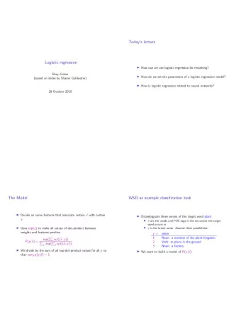
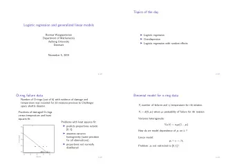
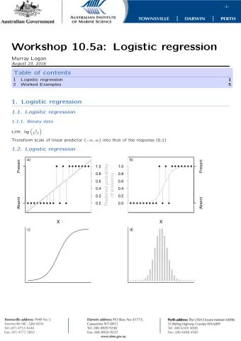
Logistic Regression GLM for binary classification sigmoid Bernoulli weights input “0” or “1” 1. Linear weights 2. sigmoid (“logistic”) function 3. Bernoulli (coin flip)
Logistic Regression GLM for binary classification sigmoid Bernoulli weights input “0” or “1” compact expression: (note when y = 1, this is equal to exp(wx)/(1+exp(wx)), which is equal to 1/(1+exp(-wx) )
Logistic Regression GLM for binary classification sigmoid Bernoulli weights input “0” or “1” compact expression: fit w by maximizing log-likelihood:
Logistic Regression geometric view p = 0.5 contour (classification boundary) neuron 2 spikes neuron 1 spikes
Bayesian Estimation three basic ingredients: 1. Likelihood jointly determine the posterior 2. Prior L (ˆ “cost” of making an estimate θ , θ ) 3. Loss function if the true value is • fully specifies how to generate an estimate from the data Bayesian estimator is defined as: Z ˆ L (ˆ θ ( m ) = arg min θ , θ ) p ( θ | m ) d θ “Bayes’ risk” ˆ θ
Typical Loss functions and Bayesian estimators L (ˆ θ , θ ) = (ˆ θ − θ ) 2 1. squared error loss 0 need to find minimizing the expected loss: Differentiate with respect to and set to zero: “posterior mean” also known as Bayes’ Least Squares (BLS) estimator
Typical Loss functions and Bayesian estimators L (ˆ θ , θ ) = 1 − δ (ˆ “zero-one” loss θ − θ ) 2. (1 unless ) 0 expected loss: which is minimized by: • posterior maximum (or “mode”). • known as maximum a posteriori (MAP) estimate.
Recommend
More recommend
Explore More Topics
Stay informed with curated content and fresh updates.

![Self-Organization in Autonomous Sensor/Actuator Networks [SelfOrg] Dr.-Ing. Falko Dressler](https://c.sambuz.com/931178/self-organization-in-autonomous-sensor-actuator-networks-s.webp)

