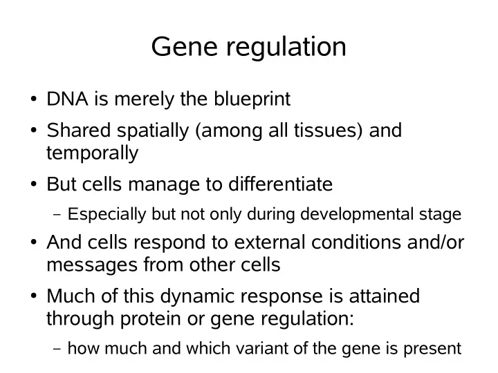
Gene regulation DNA is merely the blueprint Shared spatially (among - PowerPoint PPT Presentation

Gene regulation ● DNA is merely the blueprint ● Shared spatially (among all tissues) and temporally ● But cells manage to differentiate – Especially but not only during developmental stage ● And cells respond to external conditions and/or messages from other cells ● Much of this dynamic response is attained through protein or gene regulation: – how much and which variant of the gene is present

The central dogma

Mechanisms of gene regulation ● Pre-transcription: accessibility of the gene – the chromatin structure which packs the DNA is dynamic ● Transcription: rate ● Post-transcription: mRNA degradation rate ● Translation: rate ● Post-translation: – Modifications – Rate of degradation

Transcription factors ● Bind to specific DNA sites: Transcription Factor Binding Sites ● Typically downstream effect on mRNA transcription rate

Transcription rate

Motif finding ● Motif finding is the computational problem of identifying TFBSs ● Implicit assumption: different TFBSs of the same TF should be similar to another – Hence the name motif ● Two related tasks: – Given a specific model of TF motif compiled from a known list of TFBSs find additional sites (scanning) – Identify the unknown motif given only the DNA sequences

Modelling motifs ● Discovered sites: TACGAT TATAAT ● How do we model the motif? TATAAT GATACT – important for finding additional sites TATGAT TATATT ● Consensus pattern: TATAAT – generalizes to regular expressions 1 2 3 4 5 6 A 6 4 4 ● Positional profile: C 1 1 G 1 2 T 5 5 1 6

Generative models ● Consensus pattern: each instance is a randomly mutated version of the consensus – substitution only: the same TF binds to the various sites, so indels are unlikely to occur as the DNA-TF contact region remains the same ● Profile: instances are drawn according to the probability implied by the positional profile assuming each position is drawn independently – Pseudocounts are typically added to avoid excluding unseen letters

Counts to frequencies profile 1 2 3 4 5 6 A 6 4 4 C 1 1 G 1 2 T 5 5 1 6 1 2 3 4 5 6 A 0.1 0.7 0.1 0.5 0.5 0.1 C 0.1 0.1 0.2 0.1 0.2 0.1 G 0.2 0.1 0.1 0.3 0.1 0.1 T 0.6 0.1 0.6 0.1 0.2 0.7 What is the pseudocount in this example?

1 The fitness of a TFBS • How well does a putative TFBS w fits the model? • For a consensus model we typically use s C ( w ) = d H ( C, w ) , the Hamming distance to the consensus pattern C . • It is convenient to work with but more appropriate for uniform nucleotide sample • For a profile parametrized by M = ( f ik ) i =1: l,k =1:4 , it is natural to use the likelihood score: s M ( w ) = P M ( w ) = � l i =1 f iw i • Better: use the LLR (loglikelihood ratio) score l s M ( w ) = log P M ( w ) log f iw i � P B ( w ) = , b w i i =1 where B specifies an iid background model with nucleotide frequency ( b k ) 4 1 , typically taken from the organism or the scanned sample

2 Scanning for TFBS • Given a parametrized motif model and an associated fitness function looking for additional sites is algorithmically trivial • However, setting a cutoff score typically requires carefully analyzing the FP rates • These FP rates are set using a model of random sequences • Markov chains • shuffling • using random chunks of DNA

3 Motif finding • Do these sequences share a common TFBS? • tagcttcatcgttgacttctgcagaaagcaagctcctgagtagctggccaagcgagc tgcttgtgcccggctgcggcggttgtatcctgaatacgccatgcgccctgcagctgc tagaccctgcagccagctgcgcctgatgaaggcgcaacacgaaggaaagacgggacc agggcgacgtcctattaaaagataatcccccgaacttcatagtgtaatctgcagctg ctcccctacaggtgcaggcacttttcggatgctgcagcggccgtccggggtcagttg cagcagtgttacgcgaggttctgcagtgctggctagctcgacccggattttgacgga ctgcagccgattgatggaccattctattcgtgacacccgacgagaggcgtccccccg gcaccaggccgttcctgcaggggccaccctttgagttaggtgacatcattcctatgt acatgcctcaaagagatctagtctaaatactacctgcagaacttatggatctgaggg agaggggtactctgaaaagcgggaacctcgtgtttatctgcagtgtccaaatcctat

4 If only life could be that simple • The binding sites are almost never exactly the same • A more likely sample is: tagcttcatcgttgactttTGaAGaaagcaagctcctgagtagctggccaagcgagc tgcttgtgcccggctgcggcggttgtatcctgaatacgccatgcgccCTGgAGctgc tagaccCTGCAGccagctgcgcctgatgaaggcgcaacacgaaggaaagacgggacc agggcgacgtcctattaaaagataatcccccgaacttcatagtgtaatCTGCAGctg ctcccctacaggtgcaggcacttttcggatgCTGCttcggccgtccggggtcagttg cagcagtgttacgcgaggttCTaCAGtgctggctagctcgacccggattttgacgga CTGCAGccgattgatggaccattctattcgtgacacccgacgagaggcgtccccccg gcaccaggccgttcCTaCAGgggccaccctttgagttaggtgacatcattcctatgt acatgcctcaaagagatctagtctaaatactacCTaCAGaacttatggatctgaggg agaggggtactctgaaaagcgggaacctcgtgtttattTGCAttgtccaaatcctat

5 Searching for motifs • Simultaneously looking for a motif model and sites that will optimize a scoring function is significantly more difficult • Assume for simplicity the OOPS model (One Occurrence Per Sequence model): w m ∈ S m for m = 1 : n • A natural way to score a putative combination of a motif M and sites ( w m ) n 1 is by summing the fitness scores of all sites: n � s ( M ; w 1 , . . . , w n ) := s M ( w m ) m =1 • Thus, our goal is to search the joint space of motifs, M (consensus or profile), and alignments, w m ∈ S m , so as to optimize this score • Fortunately, for both models this can be done sequentially so we do not have to optimize simultaneously over the alignment and the motif

6 Optimizing the motif or the alignment • Once we choose the alignment, w m ∈ S m for m = 1 : n , the optimal motif for that alignment is trivial • For the consensus model it is a consensus word as it clearly minimizes the total distance to the words in the alignment • For the profile model we find with a little more effort that the best model is the one which coincides with how we define a profile: f ik = n ik n , where n ik is the number of occurrence of the letter k at position i . • Conversely, if we know the model we can find the optimal sites for the putative motif by linearly scanning the sequences • Often a motif finder will combine both the motif’s and the alignment’s optimizations and indeed they are in some sense equivalent

7 Heuristic vs. guaranteed optimizations • Assume for now l is known (we can enumerate over possible l s) and let N m be the length of S m • By considering all, roughly, � n m =1 N m gapless alignments made of w m ∈ S m we are guaranteed to find the optimal alignment under both possible motif models • Unfortunately, this number is prohibitively expensive for all but a few cases

8 Finding an optimal pattern • Consistent with our previous discussion under the OOPS model the score of a consensus word C is often the total distance : n n � � d H ( C, S m ) = w ′ ∈ S m d H ( C, w ′ ) TD ( C ) := min m =1 m =1 • Problem: find a word C that minimizes the total distance • Naive solution: enumerate all 4 l possible consensus words • Complexity: O (4 l D ) • While this approach is feasible for a larger set of parameters than the one available for alignment enumeration it is still often too expensive

9 Heuristic approaches: Sample Driven • Most of the 4 l patterns we explore in the exhaustive enumeration have little to do with our sample • Sample driven approach: compute TD ( w ) only for words w in the sample • Complexity: O ( D 2 ) where D = � n m =1 N m is the size of the sample • Analysis: • fast • but can miss the optimal pattern if it is missing from the sample • More sophisticated methods were developed based on the sample driven approach

10 CONSENSUS - greedy profile search (Hertz & Stormo ’99) • Assume the OOPS model and that l is given • There is a version that does not assume l is given (WCONSEN- SUS) • CONSENSUS Follows a greedy strategy looking first for the best alignment of just two sites: • For each i � = j , and w ∈ S i , w ′ ∈ S j compute the information content of the alignment made of w and w ′ : l 4 n ik log n ik / 2 � � I = b k i =1 k =1 • Keep the top q 2 alignments (matrices)

11 • It then greedily adds one word at a time from the sequences that are not already represented in the alignment • Let m := 3 denote the number of sequences in the current alignments • While m < n • for each of the top saved q m − 1 alignments A of m − 1 rows �� A �� compute I for all words w which come from sequences w that are not already in A • keep the best q m alignments and set m := m + 1

12 MEME (Bailey & Elkan ’94) • MEME: Multiple EM for Motif Elicitation • the multiple part is for dealing with multiple motifs • probabilistic generative model, deterministic algorithm • Recall that given the motif model we can linearly scan the sequences for instances • Conversely, given the instances deducing the profile is trivial • MEME alternates between the two tasks

13 MEME’s outline • Starting from a heuristically chosen initial profile • Sample driven: the profile is derived from the word in the sample that has a minimal total distance • MEME iterates the following two steps until convergence • score each word according to how well it fits the current profile • update the profile by taking a weighted average of all the words • The EM in MEME stands for Expectation Maximization (Dempster, Laird & Rubin ’77) which MEME’s two step procedure follows • EM is guaranteed to monotonically converge to a local maximum (intelligent choice of a starting point is crucial)