Friction, reversibility and nonequilibrium ensembles Part of the - - PowerPoint PPT Presentation

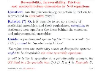
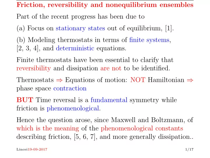
Friction, reversibility and nonequilibrium ensembles Part of the recent progress has been due to (a) Focus on stationary states out of equilibrium, [1]. (b) Modeling thermostats in terms of finite systems, [2, 3, 4], and deterministic equations. Finite thermostats have been essential to clarify that reversibility and dissipation are not to be identified. Thermostats ⇒ Equations of motion: NOT Hamiltonian ⇒ phase space contraction BUT Time reversal is a fundamental symmetry while friction is phenomenological. Hence the question arose, since Maxwell and Boltzmann, of which is the meaning of the phenomenological constants describing friction, [5, 6, 7], and more generally dissipation..

Lincei19-09-2017 1/17

One can investigate, here in the paradigmatic case of the NS, equations whether Every (even if macroscopic) dissipative evolution can be equivalent to a reversible one, provided motions are sufficiently chaotic, (usually are under large forcing or N). This generates a proposal for a general theory of equivalence between statistical descriptions of stationary states as an extension of the theory of equilibrium ensembles to nonequilibrium. [8, 9, 10], inspired by the ideas on chaos, of Ruelle and Sinai, [11, 12]. ⇒ “In microscopically reversible (chaotic) systems time reversal symmetry cannot be spontaneously broken, but only phenomenologically so”,[13]. Begin by defining “an ensemble Ec” of probab. distrib. for NS2D equation in a periodic box of size L = 1 and subject to a fix (large scale) force g, g2 = 1,e.g. only g±(2,−1) = 0

Lincei19-09-2017 2/17

for a velocity field u(x) =

k

uke−2π i k·x, uk = u−k: ˙

• u + (

u · ∂) u = −∂p + g + ν∆ u, ∂ · u = 0 (∗) The only parameter here is ν and Reynolds # is R = 1

ν.

Hence as ν varies the motion defines stationary states µC

ν

whose collection forms the viscosity ensemble Ec Conjecture: if interested in large scale observables, i.e.

• bservables depending only on the

uk with |k| < K for some arbitrary K then, in strongly chaotic regimes (i.e. R large enough), there should be other ensembles of distrib. which attribute same probability to K-local observables. Mechanism: “same” as that for equilibrium ensembles in SM, i.e. special collections of stationary states with K playing the role of the finite volume and the truncation of the equation to |k| < V playing the role, as V → ∞, of the thermodynamic limit (and ν → 0 the 0 temperature limit).

Lincei19-09-2017 3/17

In the case of the NS equations one alternative ensemble here will be the family of stationary states for the equation ˙

• u + (

u · ∂) u = −∂p + g + α( u)∆ u, ∂ · u = 0 (∗∗) α( u)

def

=

• k

k2 g

k ·

u−

k

• k

k4| u

k|2

, which have α so defined that the “dissipation” observable D(˜ u) =

• (∂˜

u(x))2dx is an exact constant of motion. Call α( u) a “reversible viscosity” (because the equations are time reversible and dissipative) Denote µM

En the stationary distr. describing statistical

properties of stationary states of new equ. with D( u) = En. We have now two “ensembles”, i.e. collections of stationary distributions, namely

Lincei19-09-2017 4/17

(1): Vary ν and let µC

ν stationary distrib. for (*) (NS2D).

Let E = µC

ν (

• (∂

u)2) = µC

ν (D(

u)) Their collection is an “ensemble” (viscosity ensemble), [∼canonical], of distr. parameterized by ν = 1

R

(2): Next consider the new equation (**): it has D( u) =

• (∂

u)2 as exact constant of motion Vary E ≡ D( u) and let µM

E station. distrib.:

ν = µM

E (α(

u)) and obtain a collection of distr. parameterized by E: this is the (enstrophy ensemble), [∼microcanonical].

Lincei09-19-2017 5/17

State µM

E labeled by E corresponds to state µC ν labeled by ν

⇒ and are equivalent, denoted µC

ν ∼ µM E , if i) OR ii) hold

i) E = µC

ν (D(·))

ii) ν = µM

E (α(·))

in the sense that they give the same statistics in the limit of large chaos to observables F which are “local observables”: i.e. depend on finitely many Fourier comp. of u. Analogy: “canonical” µC

β = “microcanonical” µM E .

Why? e.g. chaoticity implies self averaging for the

• bservable α(u) which replaces viscosity in (**):

α(u) =

• k

gk · u−k

• k |

uk|2 “self − averaging′′ to ν

Lincei09-19-2017 6/17

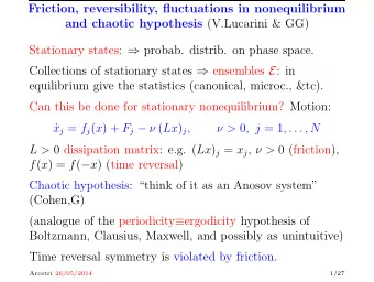
Problem: can reversibility be detected even in irrev. NS? A theoretical basis can be searched in the “Chaotic hypothesis” (GC) Chaotic hypothesis: “think of it as an Anosov system” (Cohen,G, if R is large), [14, 15, 11] which is analogous to the periodicity≡ergodicity hypothesis

• f Boltzmann, Clausius, Maxwell, and possibly as

unintuitive, [16, 17, 18]. Then in the reversible cases the phase space contraction rate σ(u)

def

= div

• α(u)∆u
• averaged over a time τ

p

def

= 1 τ τ σ(u(t) σ(·) dt (FT) should have a PDF obeying a fluctuation relation, FR, [19].

Lincei19-09-2017 7/17

This means that for large τ the probability distribution of p in µM

E (reversible viscosity ensemble) should fulfill, for some

κ (see [9, 20]). Probτ(p) Probτ(−p) = eτκ σ p+o(τ), τ → ∞ (FR) Equivalence conjecture applied to the reversible viscosity ensemble µM

E and to the observable σ(u) (which is not

constant) would imply that σ(u) fluctuates according to FR (original one!) in the corresponding µC

ν .

Of course consistency requires that the average µC

ν (α(u)) = ν

The above “predictions” can be tested. And one can explore if the equivalence conjecture can be extended even to the Lyapunov spectrum (although the Lyapunov exponents, as well as σ(u) are not local quantities).

Lincei19-09-2017 8/17

• .

FigA2-64-26-26-4-15-11.0

At 960 modes and R = 2048: the evolution of the observable “reversible viscosity”: α(u) = |k|2Fkuk |k|4|uk|2 According to the equivalence the time average of α should be

1

• R. Represents the fluctuating values of α at intervals of 104

steps (see below); the middle line is the running average of α (at intervals of 100 steps) and it converges to 1

R (horiz. line).

Lincei19-09-2017 9/17

The graph gives the values only every 1000 interaction steps (otherwise it would be just a black stain). I stress that the experiments are carried using a truncated version of the NS2D eq. with cut-off at |k| < V : the conjecture requires use of the non truncated equation, i.e. the limit V → ∞, hence it can be tested only by trying to compare stability of results with increasing V and (so far the max V reached is V = 961, but the work is in progress). We see that once the attractor might be considered reached, for instance if the running average of the reversible viscosity is close to 1

R: however wild fluctuations remain and the

statistics can be sampled to check whether the FR applies. For comparing revers. and irrevers. Lyapunov spectra it should be necessary to compute a large number time steps. This is being attempted: a few preliminary data follow

Lincei23-06-2017 10/17

It is interesting to present a few recent (mostly preliminary) results (encouraging but which need further confirmation as they are not yet very stable).

• .

FigL2-16-23-23-6-11 7.01

Local Lyapunov spectrum in a 48 modes truncation (7 × 7)

• f NS2D: (+)= viscous, (×)= reversible and R = 2048.

Lincei23-06-2017 11/17

• ✁ ✂ ✄ ✄
• ✁

• ✂

• ☎ ✁

.

FigL-32-30-30-7-17 11.01

Graph of the Lyapunov spectra in a 15 × 15 truncation for the NS2D with viscosity and reversible viscosity (captions ending respectively in 0 or 1) with (the 224 points) interpolated by lines, R = 2048. Preliminary

Lincei23-06-2017 12/17

It is interesting to look at the fluctuations of En in the irreversible NS while the Lyapunov exponents of the previous image are measured: history (unit step 131072), running average and precomputed average of En

• ✂ ✂

• ✂ ✂

• ✟

• ✎ ✏

• ✎ ✏

• ✟

• ✎ ✏

• ✎ ✏

• ✎ ✏
• ✟

• ✟

• ✎ ✏
• ✟

• ✎ ✏
• ✟ ✠
• ✟

• ✎ ✏
• .

FigEn-32-30-30-7-17 11.0

The evolution of the reversible viscosity measured in the irreversible evolution has similar behavior.

Lincei23-06-2017 13/17

Remarks: (1) The NS equations can be regarded, for large scale observables, as statistically equivalent to the motion

• f N microscopic particle subject to thermostats keeping

for instance the total energy constant. Then the microscopic motion is certainly chaotic at all R and this suggests that equivalence might hold at all R (even in the laminar regime or mildly chaotic flows where there may be several stationary states, [21]: a situation similar to the equivalence between ensembles in equilibrium and in presence of phase transitions). In other words the equivalence for R large enough might extend to all R, (but the appropriate reversible models are likely to be different in the laminar regimes). (2) The observable D( u) might not play a special role: it could be replaced by the energy

• u(x)2dx. Some evidence

for this has been found in [22] but doubts are raised in [23].

Lincei23-06-2017 14/17

(3) And, as in Statistical Mechanics, it should be possible to fix more than a single observable thus generating many equivalent ensembles. (4) The analysis applies word-by-word to NS3D: in that case it is even more interesting as there is a natural truncation at Kolmogorov scale. An important simulation, [4], has been performed on a 1283 truncation of NS3D at scale > O(R

3 4) imposing many constraints: namely the

energy content of each shell was fixed to the OK-value (following the 5

3 power law) obtaining a stationary state (at

high R) which on large scale observables is the same as the unconstrained evolution. See also [24]. (5) The conjecture here would say that fixing just one

• bservable, namely the dissipation D(u), should be

sufficient at large R for local observables statistics.

Lincei23-06-2017 15/17

(6) A final remark: since the reversible viscosity model is reversible it is tempting to try to connect the fluctuations

• f the dissipation with the “fluctuation relation”,

[15, 9, 20]. This leads to think that (a) another ensemble could be constructed replacing the viscosity with a whites Gaussian process, with average satisfying the fluctuation relation (?) (b) the fluctuations of the reversible phase space contraction observed in the irreversible evolution should be a stochastic process obeying a fluctuation relation (see Fig. above): a further way to reveal reversibility in the irreversible evolution.

Quoted references [1]

• D. J. Evans and G. P. Morriss.

Statistical Mechanics of Nonequilibrium Fluids. Academic Press, New-York, 1990. [2]

• S. Nos´

e. A unified formulation of the constant temperature molecular dynamics methods. Journal of Chemical Physics, 81:511–519, 1984. [3]

• W. Hoover.

Canonical equilibrium phase-space distributions. Physical Review A, 31:1695–1697, 1985. [4] Z.S. She and E. Jackson. Constrained Euler system for Navier-Stokes turbulence. Physical Review Letters, 70:1255–1258, 1993. [5] J.C. Maxwell. Illustrations of the dynamical theory of gases. In: The Scientific Papers of J.C. Maxwell, Cambridge University Press, Ed. W.D. Niven, Vol.1, pages 377–409, 1860. [6] J.C. Maxwell. On the dynamical theory of gases. In: The Scientific Papers of J.C. Maxwell, Cambridge University Press, Ed. W.D. Niven, Vol.2, pages 26–78, 1866. [7]

• L. Boltzmann.

Weitere Studien ¨ uber das W¨ armegleichgewicht unter Gasmolek¨ ulen. Wiener Berichte, 63, (W.A.,#22):275–370, (316–402), 1872. [8]

• G. Gallavotti.

Equivalence of dynamical ensembles and Navier Stokes equations. Physics Letters A, 223:91–95, 1996. [9]

• G. Gallavotti.

Dynamical ensembles equivalence in fluid mechanics. Physica D, 105:163–184, 1997. [10]

• D. Ruelle.

A remark on the equivalence of isokinetic and isoenergetic thermostats in the thermodynamic limit. Journal of Statistical Physics, 100:757–763, 2000. [11]

• D. Ruelle.

Turbulence, strange attractors and chaos. World Scientific, New-York, 1995.

[12]

• Ya. G. Sinai.

Topics in ergodic theory, volume 44 of Princeton Mathematical Series. Princeton University Press, 1994. [13]

• G. Gallavotti.

Breakdown and regeneration of time reversal symmetry in nonequilibrium statistical mechanics. Physica D, 112:250–257, 1998. [14]

• D. Ruelle.

Measures describing a turbulent flow. Annals of the New York Academy of Sciences, 357:1–9, 1980. [15]

• G. Gallavotti and D. Cohen.

Dynamical ensembles in stationary states. Journal of Statistical Physics, 80:931–970, 1995. [16]

• G. Gallavotti.

Ergodicity: a historical perspective. equilibrium and nonequilibrium.

• Eur. Phys. J. H., 41, online-first:1–80, 2016.

[17]

• G. Gallavotti.

Nonequilibrium and irreversibility. Theoretical and Mathematical Physics. Springer-Verlag and http://ipparco.roma1.infn.it & arXiv 1311.6448, Heidelberg, 2014. [18]

• D. Ruelle and F. Takens.

On the nature of turbulence. Communications in Mathematical Physics, 20:167–192, 1971. [19]

• G. Gallavotti and D. Cohen.

Dynamical ensembles in nonequilibrium statistical mechanics. Physical Review Letters, 74:2694–2697, 1995. [20]

• F. Bonetto and G. Gallavotti.

Reversibility, coarse graining and the chaoticity principle. Communications in Mathematical Physics, 189:263–276, 1997.

[21]

• V. Franceschini, C. Tebaldi, and F. Zironi.

Fixed point limit behavior of N-mode truncated Navier-Stokes equations as N increases. Journal of Statistical Physics, 35:387–397, 1984. [22]

• G. Gallavotti, L. Rondoni, and E. Segre.

Lyapunov spectra and nonequilibrium ensembles equivalence in 2d fluid. Physica D, 187:358–369, 2004. [23]

• L. Rondoni and C. Mejia-Monasterio.

Fluctuations in nonequilibrium statistical mechanics: Models, mathematical theory, physical mechanisms. Nonlinearity, 20:R1, 2007. [24]

• L. Fang, J.T.W. Bos, L. Shao, and JP. Bertoglio.

Time reversibility of NavierStokes turbulence and its implication for subgrid scale models. Journal of Turbulence, page 114, 2012. Also: http://arxiv.org & http://ipparco.roma1.infn.it Slides, edited, of the talk at the confrence “Advances in Mathematics and Theoretical Physics”, Roma, Accademia dei Lincei, 19-21 Sept. 2017.

• n 19 Sept 2017.