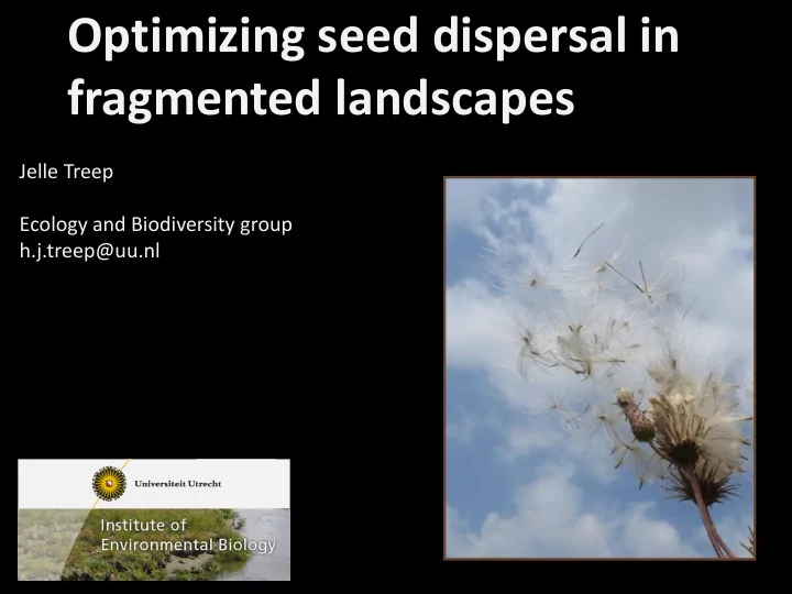
fragmented landscapes Jelle Treep Ecology and Biodiversity group - PowerPoint PPT Presentation
Optimizing seed dispersal in fragmented landscapes Jelle Treep Ecology and Biodiversity group h.j.treep@uu.nl Background: Master Computational Geo-ecology (UvA) Movement and dispersal Ecology Atmospheric sciences PhD Ecology and
Optimizing seed dispersal in fragmented landscapes Jelle Treep Ecology and Biodiversity group h.j.treep@uu.nl
Background: Master Computational Geo-ecology (UvA) Movement and dispersal Ecology Atmospheric sciences
PhD Ecology and Biodiversity “Flying, floating or hitching a ride: The dispersal of plants in heterogeneous landscapes.”
Contents Part 1: Mechanistic modelling seed dispersal by wind Part 2: Timing of dispersal Part 3: Optimal dispersal
Seed dispersal • Colonisation • Gene flow • Range shifts • Nature restoration • Habitat loss and fragmentation • Environmental change
Seed dispersal • Habitat loss and fragmentation 1900 1950 2000
Seed dispersal • Nature restoration
Dispersal kernel Lippe et al. 2013
Traits
Obtaining dispersal kernels Observations
Obtaining dispersal kernels Fascinating results!! However, can we extrapolate this kernel to other situations? • Wind? • Surrounding vegetation? • Species traits? Therefore: mechanistic modelling
Mechanistic modelling • Simple complex Simple model 𝑰 𝐲 = 𝒗 𝒙 𝒕 Okubo & Levin, 1989
• Simple complex Stochastic turbulence 𝒚 (𝒖+𝟐) = 𝒚 (𝒖) + 𝒗 + 𝒗 , 𝒛 (𝒖+𝟐) = 𝒛 (𝒖) + 𝒘 , 𝒜 (𝒖+𝟐) = 𝒜 (𝒖) + 𝒙 , + 𝑿 𝒕 CELC Katul and Albertson, 1998
• Simple complex Stochastic turbulence
Mechanistic modelling • Simple complex Large Eddy Simulations RAFLES Bohrer et al., 2008
Mechanistic modelling • Simple complex Large Eddy Simple model Simulations Stochastic turbulence • Question and Scale dependent!!! • Time scale and spatial scale • Computational limits
Discussion Closer to reality? Uncertainty
Contents Part 1: Mechanistic modelling seed dispersal by wind Part 2: Timing of dispersal Part 3: Optimal dispersal
Adaptive traits • Seed release height H • Seed terminal velocity Ws
Timing May shape entire dispersal distribution
Wind Thermals Soons & Bullock, 2008 Maurer, 2013
Timing of seed dispersal in wind-dispersed plant species . Frequency wind Frequency seed abscission Pazos et al. 2013
Timescales of seed abscission • Threshold drag force (milliseconds) • Material fatigue (minutes – hours) • Ripening (hours – days)
Waiting may be risky Seed predation Rain
AIM Build a framework to study non-random seed abscission strategies across timescales QUESTIONS • Which timescales are important in the timing of seed dispersal? • What are the consequences of non-random seed release for dispersal kernels?
Field study m u Leontodon hispidus c a i t n a r u a m u i c a r e i H Observation time June 10 - October 3 May 26 - October 3 Seed terminal velocity in m s -1 0.3 0.9 Number of seeds per inflorescence 50 77 Number of plants 24 34 Number of observations 2633 6427
Field study
Coupled Eulerian-Lagrangian Closure model (CELC, Katul et al. 1998) Wind Turbulence (x) Turbulence (y) Turbulence (z) Dissipation
Input Wind speeds (0-20 m/s) Random turbulence CELC Seed trajectories Output Input Dispersal kernels for each wind speed (0-20 m/s) KNMI data Dynamic Wind Input KNMI data Dispersal wind and precipitation model Precipitation Output Dispersal kernels for different sigmoid functions
Dynamic dispersal model Assumptions Seed production constant Probability of abscission Disturbance p(a) = 1 / (1 + e (- α (u- β )) ) 99 percentile dispersal distance
Dispersal kernels
Results: 99 percentile dispersal distance
Results Without disturbance
Results Without disturbance With disturbance
Conclusions • By non-random seed release, plants may increase the tail of the dispersal kernel (99-percentile by 40 %) • Risks prevent a too strong selection for high wind speeds • Both model and field study indicate strong biased seed abscission at wind speeds above 5-6 m s -1
Conclusions • Mechanistic models are flexible tools to estimate dispersal kernels • However, tail of the dispersal kernel is still underestimated • Possibly a better representation of traits may improve estimations > evolutionary insights? 𝑰 𝐲 = 𝒗 𝒙 𝒕
Contents Part 1: Mechanistic modelling seed dispersal by wind Part 2: Timing of dispersal Part 3: Optimal dispersal
Mechanistic perspective versus evolutionary perspective how dispersal determines fitness of individuals and populations remains unclear
What is optimal? Maximize fitness: Nearest unoccupied location? • Competition • Density dependent mortality • Facilitation • Habitat fragmentation Janzen-Connell hypothesis
Analogy to movement ecology Dispersal is a search Humphries et al. 2014
Random walks Lévy versus Brownian 𝑞 𝑚 = 𝑚 −𝜈 Viswanathan et al. 1999
Random walks Lévy versus Brownian Remember: Low μ < 2 more LDD Intermediate μ ≈ 2 Levy High μ ≥ 3 less LDD Viswanathan et al. 1999
Lévy walks optimize the search efficiency in random searches Search efficiency = average distance traveled before finding target Koelzsch et al. 2015 De Jager et al. 2011 Raichlen et al. 2014
Finding the nearest unoccupied location? Reynolds et al. 2012
Does the comparison between animals and plants hold?
Aim • Identify a null model for optimal seed dispersal strategies in plants • Assess how dispersal strategies may maximize species survival in landscapes that differ in terms of fragmentation and dynamics
Landscape Species 1 Species 2 Unsuitable
Dispersal
Semelparous species Each generation all individuals disperse an equal amount of seeds Species 1 Species 2
Stochastic colonization of a grid cell based on expected seed arrival of both species Species 2 Species 1 6 4
Landscapes Landscape parameters Patch size 1, 2, 4, 8, 16, 32, 64, 128 Interpatch distance 1, 5, 10, 50, 100, 500, 1000 Patch turnover rate 0, 0.01, 0.05, 0.1, 0.5, 1
Example run
Pairwise invasibility plot Homogeneous landscape
Pairwise invasibility plot Patchsize 8 | Interpatch distance 50 | Patch turnover 0.1
Metrics Patchsize 8 | Interpatch distance 50 | Patch turnover 0.1
Patchsize 8 | Patch turnover 0.01 Interpatch distance 12 Interpatch distance 50 Interpatch distance 100 Interpatch distance 500
Patch turnover 0.01
Patch turnover 0.1 Interpatch distance Interpatch distance
Conclusions • In homogeneous or random unpredictable landscapes uniform dispersal is optimal • In patchy environments it depends on the interpatch distance whether seeds need to be dispersed closeby or whether an intermediate (Lévy-like) strategy is better • In dynamic landscapes it is generally better to increase the tail of the dispersal kernel
Conclusions • When all other plant traits are equal, plants can outcompete other plants by optimizing the shape of dispersal kernels • Optimal dispersal strategy largely depends on landscape • Dispersal traits can evolve when landscape parameters are relatively constant over time
Contents Part 1: Modelling seed dispersal by wind Part 2: Optimal dispersal Part 3: Timing
Questions? h.j.treep@uu.nl
Recommend
More recommend
Explore More Topics
Stay informed with curated content and fresh updates.
