Forecasting General problem: predict x n + m given x n , x n 1 , . - PowerPoint PPT Presentation

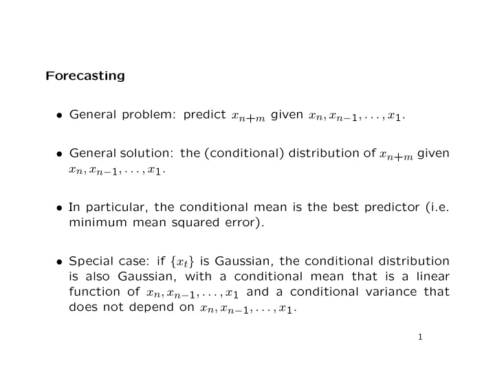
Forecasting • General problem: predict x n + m given x n , x n − 1 , . . . , x 1 . • General solution: the (conditional) distribution of x n + m given x n , x n − 1 , . . . , x 1 . • In particular, the conditional mean is the best predictor (i.e. minimum mean squared error). • Special case: if { x t } is Gaussian, the conditional distribution is also Gaussian, with a conditional mean that is a linear function of x n , x n − 1 , . . . , x 1 and a conditional variance that does not depend on x n , x n − 1 , . . . , x 1 . 1

Linear Forecasting • What if x t is not Gaussian? • Use the best linear predictor: x n n + m . • Not the best possible predictor, but computable. 2

One-step Prediction • The hard way: suppose x n n +1 = φ n, 1 x n + φ n, 2 x n − 1 + · · · + φ n,n x 1 . • Choose φ n, 1 , φ n, 2 , . . . , φ n,n to minimize the mean squared pre- �� � 2 � x n +1 − x n diction error E . n +1 • Differentiate and equate to zero: n linear equations in the n unknowns. • Solve recursively (in n ) using the Durbin-Levinson algorithm. Incidentally, the PACF is φ n,n . 3

One-step Prediction for an ARMA Model • The easy way: suppose we can write x n +1 = some linear combination of x n , x n − 1 , . . . , x 1 + something uncorrelated with x n , x n − 1 , . . . , x 1 . • Then the first part is the best linear predictor, and the second part is the prediction error. • E.g. AR( p ) , p ≤ n : x n +1 = φ 1 x n + φ 2 x n − 1 + · · · + φ p x n +1 − p + w n +1 . � �� � � �� � second part first part 4

General ARMA case • Now x n +1 = φ 1 x n + φ 2 x n − 1 + · · · + φ p x n +1 − p + θ 1 w n + θ 2 w n − 1 + · · · + θ q w n +1 − q + w n +1 . • First part on the right hand side is a linear combination of x n , x n − 1 , . . . , x 1 . • Last part, w n +1 , is uncorrelated with x n , x n − 1 , . . . , x 1 . 5

• Middle part? If the model is invertible, w t is a linear com- bination of x t , x t − 1 , . . . , so if n is large, we can truncate the sum at x 1 , and w n , w n − 1 , . . . , w n +1 − q are all (approximately) linear combinations of x n , x n − 1 , . . . , x 1 . • So the middle part is also approximately a linear combination of x n , x n − 1 , . . . , x 1 , whence x n n +1 = φ 1 x n + φ 2 x n − 1 + · · · + φ p x n +1 − p + θ 1 w n + θ 2 w n − 1 + · · · + θ q w n +1 − q and w n +1 is the prediction error, x n +1 − x n n +1 . 6

Multi-step Prediction • The easy way: build on one-step prediction. E.g. two-step: x n +2 = φ 1 x n +1 + φ 2 x n + · · · + φ p x n +2 − p + θ 1 w n +1 + θ 2 w n + · · · + θ q w n +2 − q + w n +2 . • Replace x n +1 by x n n +1 + w n +1 : x n +2 = φ 1 x n n +1 + φ 2 x n + · · · + φ p x n +2 − p + θ 2 w n + · · · + θ q w n +2 − q + w n +2 + ( φ 1 + θ 1 ) w n +1 . 7

• The first two parts are again (approximately) linear combi- nations of x n , x n − 1 , . . . , x 1 , and the last is uncorrelated with x n , x n − 1 , . . . , x 1 . So x n n +2 = φ 1 x n n +1 + φ 2 x n + · · · + φ p x n +2 − p + θ 2 w n + · · · + θ q w n +2 − q and the prediction error is x n +2 − x n n +2 = w n +2 + ( φ 1 + θ 1 ) w n +1 . • Note that the mean squared prediction error is � 1 + ( φ 1 + θ 1 ) 2 � σ 2 ≥ σ 2 w . w Mean squared prediction error increases as we predict further into the future. 8

Forecasting with proc arima • E.g. the fishery recruitment data. • proc arima program and output. • Note that predictions approach the series mean, and “std errors” approach the series standard deviation. 9

• The “autocorrelation test for residuals” is borderline, largely because of residual autocorrelations at lags 12, 24, . . . . • Spectrum analysis shows that these are caused by seasonal means, which can be removed: proc arima program and output. 10