for Speech Synthesis and Sensor Data Augmentation Deep Generative - PowerPoint PPT Presentation

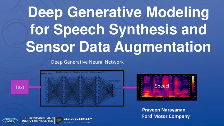
Deep Generative Modeling for Speech Synthesis and Sensor Data Augmentation Deep Generative Neural Network Speech Text Praveen Narayanan Ford Motor Company

PROJECT DESCRIPTION  Use of DNNs increasingly prevalent as a solution for many data intensive applications  Key bottleneck – requires large amounts of data with rich feature sets => Can we produce synthetic, realistic data?  This work aims to leverage state of the art DNN approaches to produce synthetic data that are real world representative • Deep Generative modeling: − A new research approach using DNN, came into vogue in the last three years − Examples: VAE, GAN, PixelRNN, Wavenet • VAE – Variational Autoencoder: Maximizing a variational objective bound + reparametrization • GAN – Generative Adversarial Nets: Adversarial learning with a discriminator  Some application areas of generative models: • Data augmentation in missing data problems – e.g. when labels are missing or bad • Generating samples from high dimensional pdfs – e.g. producing rich feature sets • Synthetic data generation for simulation – e.g. reinforced learning in a simulated environment 2

TECHNICAL SCOPE  Text to speech problem Hello • Given text, convert to speech • Use to train ASR Nǐ huì shuō  Produce speech from text with custom attributes pǔtōnghuà Examples: ma Male vs female speech (voice conversion) Accented speech: English in different accents Do you Multilanguage speak Mandarin Mandarin  Sensor data augmentation ? • Effecting transformations on data Parrot − Rotations on point clouds − Generating data in adverse weather conditions Accent 3

SCOPE OF THIS TALK  Very brief introduction to generative models (GANs, VAEs, autoregressive models)  Describe the text to speech problem (TTS)  High level overview of “ Tacotron ” – a quasi end to end TTS system from google  Speech feature processing • Different types of features used in speech signal processing  Describe the CBHG network and our implementation • Originally proposed in the context of NMT • Used in Tacotron  Voice conversion using VAEs  Conditional variational autoencoders to transform images

GENERATIVE MODELING “TOOLS”  Generative Adversarial Networks (GANs)  Variational Autoencoders (VAEs)  Autoregressive models • RNNs − Vanilla RNNs pix2pix − Gated: LSTM, GRU, possibly bidirectional − Seq2seq + attention • Dilated convolutions − Wavenet, Bytenet, PixelRNN, PixelCNN [Goodfellow; Kingma and Welling; Rezende and Mohamed; Van den Oord et al] DRAW PixelRNN

VARIATIONAL AUTOENCODER RESOURCES Vanilla VAE  Kingma and Welling  Rezende and Mohamed Semi Supervised VAE (SSL+conditioning, etc.)  Kingma et. al Related  DRAW (Gregor et al)  IAF/Variational Normalizing flows (Kingma, Mohamed) Blogs and helpers  Tutorial on VAEs (Doersch)  Brian Keng’s blog (http://bjlkeng.github.io/)  Shakir Mohamed’s blog (http://blog.shakirm.com /)  Ian Goodfellow’s book (http://www.deeplearningbook.org/)

TEXT TO SPEECH  Given a text sequence, produce a speech sequence using DNNs  Historical approach: • Concatenative TTS (concatenate speech segments) • Parametric TTS (Zen et al) − HMMs − DNNs  Recent developments • Treat as seq2seq problem a la NMT  Two current approaches • RNNs • Autoregressive CNNs (Wavenet/Bytenet/PixelRNN)

CURRENT BLEEDING EDGE LANDSCAPE  Last 2 years (!) • Baidu DeepVoice series (2016, 2017, 2018) • Tacotron series (2017+) • DeepVoice, Tacotron are seq2seq models with text in => waveform out − Seq2seq + attention (Bahdanau style) • Wavenet series [not relevant, but very instructive] − Wavenet 1: fast training, slow generation − Wavenet 2: (a brilliancy) – two developments (100X over wavenet) 1) Inverse Autoregressive Flow – fast inference 2) Probability Density “Distillation” (as against estimation) • cooperative training during inference to match PDF of trained wavenet

DNN WORKFLOW Deep Generative Neural Network  Tacotron, Baidu Deepvoice • Google (2017), Tacotron (2016, 2017) Speech • Seq2seq+attention RNN trained end to end Speech Text to Speech Speech DNN Text Features spectrogram waveform Seq2seq hello Attention RNN

TEXT VS PHONEME FEATURES Earlier models h/eh/l/ow RNN Speech hello RNN Text Phoneme sequence sequence Phoneme (‘token’/segment) > text Tacotron Text=>phoneme needs another DNN Not totally “end -to- end” hello RNN Speech Text Speech frames sequence

SEQ2SEQ+ATTENTION  Originally proposed in NMT context (Bahdanau, Cho et. al.) Variable word length I am not a small black cat Word ordering different je ne suis pas un petit chat noir Attention weights Input and output words

TACOTRON: SEQ2SEQ+ATTENTION Mel Tacotron Text Spectrogram Processed text sequence Output mel frames Sophisticated architecture Built on top of Bahdanau Preprocessing of text Postprocessing of output ‘ mel ’ frames Training: <text/mel> pairs

AUDIO FEATURES FOR SPEECH DNNS  Main theme: Synthesize voice using generative modeling (VAEs/GANs)  Sub-theme: Feature generation for audio critical for audio processing  Audio representations: • Raw waveforms: uncompressed , 1D , amplitude vs time – 16 kHz • Linear spectrograms: 2D , frequency bins vs time (1025 bins) • Mel spectrograms: 2D, compressed log-scale representation (80 bins)  Compressed (mel) representations • Easier to train neural network • Lossy • Need compression but also need to keep sufficient number of features

MOTIVATION Power & mel spectrogram Speech ? Speech DNN Text Features Text to Speech Speech Speech ? Speech DNN STFT Speech Features Features Raw Audio Speech to transformed speech

MEL FEATURES  Order of magnitude compression beneficial to train DNNs • Linear spectrograms: 1025 bins • Mel: 80 bins  Energy is mostly contained in a smaller set of bins in linear spectrogram  Creating mel features • Low frequencies matter – closely spaced filters • Higher frequencies less important – larger spacing (Kishore Prahllad, CMU) 𝑁 = 1125 ln(1 + 𝑔 700) Linearly spaced bins in mel scale Bins closely spaced at lower frequencies

AUDIO PROCESSING WORKFLOW 1025 80 Mel Feature Linear Audio Spectrogram Generation Spectrogram Mel Linear Training Mel VAE Mel Speech data Spectrogram Network Spectrogram Linear Postprocessing Mel Audio PostNet Spectrogram To recover audio Spectrogram

POST PROCESSING TO RECOVER AUDIO  Use of Griffin-Lim procedure to convert from linear spectrogram to waveform 80 1025 Conv bins bins 80 FilterBank BiLSTM bins Highway Processed Mel frames Linear PostNet Need to use a postprocessing DNN To recover audio waveform Griffin Audio Lim

CBHG/POSTNET  Originally, in Tacotron (adapted from Lee et. al.)  “Fully Character -Level Neural Machine Translation without Explicit Segmentation”  Tacotron: text=>phoneme bypassed to allow text=>speech (Tacotron)  Used in 2 places: • Encoder: Text=>text features • Postprocessor net • Mel spectrogram => linear spectrogram (=>audio)

CBHG DESCRIPTION  Conv+FilterBank+Highway+GRU  Take convolutions of sizes (1,3,5,7, etc.) to account for words of varying size  Pad accordingly to create stacks of equal length  Max pool to create segment embeddings (Lee et al) Pool (stride=1) convolutions

CBHG DESCRIPTION  Send to highway layers (improves training deep nets – Srivastava)  Bi-directional GRU or LSTM GRU GRU

HIGHWAY LAYERS OVERVIEW  Improves upon residual connections  Residual: • 𝑧 = 𝑔 𝑦 + 𝑦  Highway motivation: use fraction of input • 𝑧 = 𝑑. 𝑔 𝑦 + 1 − 𝑑 . 𝑦 Srivastava et al  Now make ‘c’ a learned metric • 𝑧 = 𝑑 𝑦 𝑔 𝑦 + 1 − 𝑑 𝑦 . 𝑦  Make c(x) lie between 0 and 1 by passing through sigmoid unit  Finally, use a stack of highway layers. E.g. y1(x), y2(y1), y3(y2), y4(y3)

SPECTROGRAM RECONSTRUCTIONS  Use filter sizes of 1, 3, 5 in CBHG  Use bi-LSTM  Highway layer stack of 4  Input: 80 bin mel frames with seq length 44  Output: 1025 bin linear frames with seq length 44  PyTorch  Librosa

SAMPLES “ground truth” “reconstructed”

SAMPLES Ground truth Reconstruction

GENERATIVE MODELING WITH VARIATIONAL AUTOENCODERS DESIDERATA

GENERATIVE MODELING WITH VARIATIONAL AUTOENCODERS  Variational Inference fashioned into DNN (Kingma and Welling; Rezende and Mohamed) Reconstruction Input Latent

PROPERTIES OF VAE  Feed input data and encode representations in reduced dimensional space  Reconstruct input data from reduced dimensional representation • Compression  Generate new data by sampling from latent space Input Reconstruction Training Latent Encoder Decoder Layer Inference Sample Generation Latent Decoder Layer N(0,I)

RECONSTRUCTIONS Original Image: 560 pixels Reconstructed from 20 latent variables 28X image compression advantage Ground Truth Reconstruction

GENERATION Faces and poses that did not exist!

APPLICATIONS SPEECH ENCODINGS