Flood risk management methodology for Lakes and adjacent areas: The - PowerPoint PPT Presentation
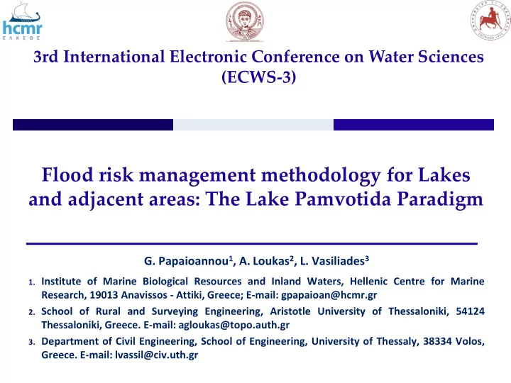
3rd International Electronic Conference on Water Sciences (ECWS-3) Flood risk management methodology for Lakes and adjacent areas: The Lake Pamvotida Paradigm G. Papaioannou 1 , A. Loukas 2 , L. Vasiliades 3 1. Institute of Marine Biological
3rd International Electronic Conference on Water Sciences (ECWS-3) Flood risk management methodology for Lakes and adjacent areas: The Lake Pamvotida Paradigm G. Papaioannou 1 , A. Loukas 2 , L. Vasiliades 3 1. Institute of Marine Biological Resources and Inland Waters, Hellenic Centre for Marine Research, 19013 Anavissos - Attiki, Greece; E-mail: gpapaioan@hcmr.gr 2. School of Rural and Surveying Engineering, Aristotle University of Thessaloniki, 54124 Thessaloniki, Greece. E-mail: agloukas@topo.auth.gr 3. Department of Civil Engineering, School of Engineering, University of Thessaly, 38334 Volos, Greece. E-mail: lvassil@civ.uth.gr
Objectives Floods are one of the most devasting natural hazards with high mortality percentage, destruction of infrastructure and large financial losses. According to the EU Flood Directive (Directive 2007/60/EC), several scenarios should be investigated such as scenarios with low, medium and high probability of flooding (eg: T = 50, 100, 1000 years). This study presents a methodological approach for flood risk management at lakes and adjacent areas that is based on the implementation of the EU Floods Directive (2007/60/EC) in Greece. Contemporary engineering approaches have been used for the estimation of the inflow hydrographs. The hydraulic-hydrodynamic simulations implemented in the following order: a) hydrologic modelling of lake tributaries and estimation flood flow inflow to the lake, b) flood inundation modelling of lake tributaries, c) simulation of the lake as a closed system, d) simulation of the lake outflows to the adjacent areas, e) simulation of flood inundation of rural and urban areas adjacent to the lake. 3rd International Electronic Conference on Water Sciences (ECWS-3) ,15-30 November 2018
Flood inundation modelling for lakes and adjacent areas The main goal is to highlight the possible disastrous effect of fluvial floods on human health, economic activities, cultural heritage, and the environment for three typical design return periods (T = 50, 100, 1000 years), according to the European Union Flood Directive 2007/60/EC and the respective Greek legislation. Flood risk management methodological framework for lakes and adjacent areas : The single event-based deterministic approach is adopted, based on three modelling components: a synthetic storm generator/estimator; i. a hydrological simulation model; and ii. a hydraulic simulation model. iii. Basic assumptions: The flood hazard is connected to the determination of the input rainfall return period. Results: Flood hazard maps (for T = 50, 100, 1000 years) corresponding to the “average” hydrological scenario as well as two “extreme” scenarios, which allow providing lower and upper uncertainty bounds of the estimated flood quantities for each return period of interest. The proposed framework is described in the next paragraphs. 3rd International Electronic Conference on Water Sciences (ECWS-3) ,15-30 November 2018
Synthetic Design Storm Estimator Basic assumption : Flood risk is determined in terms of return period, T, of the design rainfall (hyetograph). Several rainfall scenarios investigated, setting D = 24 h (which is about five times larger than the time of concentration of the basin) and Δ t = 15 min. Semi-distributed approach - Spatially-varying rainfall inputs across sub-basins, thus accounting for the heterogeneity of the storm regime over the study basin, which is due to climatic reasons as well as relief and orography effects. The computational procedure for extracting design hyetographs across sub-basins comprised three steps: estimation of partial rainfall depths for all temporal scales and return periods of interest, a) on the basis of spatially-averaged Intensity Duration Frequency (IDF) curves relationships; derivation of a synthetic hyetograph, by placing the partial depths at specific time b) intervals across the given duration (i.e., 24 h); and application of an empirical reduction formula, to transform point to areal estimations. c) The IDF relationships could be described by the following equation, proposed by (Koutsoyiannis et al., 1998): i ( d , T ) = λ ΄ ( Τ κ – ψ ΄) / (1 + d / θ ) η where λ ΄, ψ ΄, κ , θ and η are parameters that were estimated using a stepwise approach (Monte Carlo approach, Tyralis et al., 2013). 3rd International Electronic Conference on Water Sciences (ECWS-3) ,15-30 November 2018
Hydrological Modelling For each return period of interest ( T = 50, 100, 1000 years ), three scenarios (herein referred to as low, average and high ) have been formulated, in order to account for joint rainfall and hydrological uncertainties. Specifically, the design rainfall estimation provided by the IDF relationship is assumed to correspond to the average scenario (or median 50%), while its 80% confidence limits, which are measure of rainfall uncertainty, correspond to the two extreme scenarios (e.g. low-20% and high-80%) (Efstratiadis et al., 2014) . The design hyetorgraphs have been produces by IDF curves using the Alternating Block Method (ABM) for return periods of T=50 and 100 years, and the method of Worst Case Design Storm (WCDS) for the return period of T=1000 years. Hydrological uncertainty has been expressed in terms of three typical antecedent soil moisture conditions (dry, moderate, wet ). SCS-CN approach (SCS, 1972) used for the estimation of excess rainfall. Antecedent soil moisture conditions: the dry (or low ) represented by CNI , a) the moderate (or average ) represented by CNII , b) and the wet (or high ) represented by CNIII . and transformation of the hyetograph to c) flood runoff. The transformation of the excess rainfall over the basin to flood hydrograph at the outlet junction is made by using the dimensionless curvilinear unit hydrograph approach of SCS of the HEC-HMS modelling system. 3rd International Electronic Conference on Water Sciences (ECWS-3) ,15-30 November 2018
Hydraulic-Hydrodynamic Modelling Under complex and composite flow conditions and wide flood plains, a 2D-modelling approach is generally suggested due to the provision of more accurate or realistic results (Papaioannou et al., 2016). Therefore, the two dimensional (2D) HEC-RAS model is used for the hydraulic/hydrodynamic flow simulation and flood routing within streams/rivers and lakes. Digital Elevation Model (DEM) processing (pixel size = 5m) : Digital Surface Models (DSM) that derived from 1:5000 aerial photos was merged Total DSM has been processed to fill/sink the erroneous areas The final DSM has been re-corrected using typical elevation downgrading methods for the DEM generation Roughness coefficient estimation - CORINE land cover data and standard roughness coefficient tables (e.g. Dimitriadis et al., 2016) Based on EU Flood Directive guides the “upper” and “lower” boundaries of Manning’s roughness coefficient were estimated, as − 50% and +50% of the average Manning’s roughness coefficient values, respectively. Hydraulic structures detection through: a) Aerial photographs, b) A GIS database of the technical works, c) Field observations and d) Information collected by several authorities. 3rd International Electronic Conference on Water Sciences (ECWS-3) ,15-30 November 2018
Hydraulic-Hydrodynamic Modelling Flood protection works and the geometry of all hydraulic structures incorporated to the final DEM A basic concern in flood inundation modelling of urban and suburban areas is the building representation within the 2D hydraulic-hydrodynamic model Urban and suburban areas flood inundation modelling component: The main methodologies followed for the representation of the built up areas are: (a) The cells of the mesh that are within a building block area are defined as solid object. (b) The cells of the mesh that are within a building block area are assigned with big elevation values in order to work as a blocked area. (c) The cells of the mesh that are within a building block area are assigned with big roughness coefficient values. Recent studies that investigated the building block representation methods showed that all techniques have disadvantages and advantages and none of them prevail among the others (Bellos and Tsakiris, 2015). Therefore, the second building block representation methodology is followed in this study for large urban areas (cities) and the third method for suburban areas and small settlements (villages) based on the modelling simulation time and the scale (large scale applications) of the proposed framework. 3rd International Electronic Conference on Water Sciences (ECWS-3) ,15-30 November 2018
Recommend
More recommend
Explore More Topics
Stay informed with curated content and fresh updates.
