First order optimization. Last time. Other scenarios. min f ( x ) - PowerPoint PPT Presentation

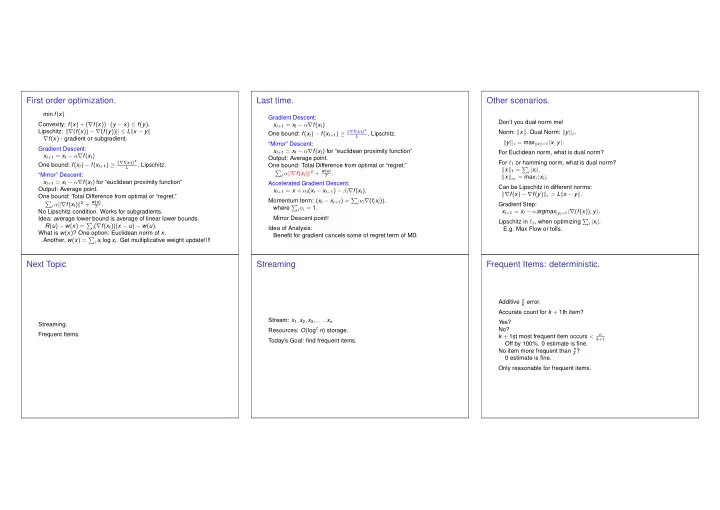
First order optimization. Last time. Other scenarios. min f ( x ) Gradient Descent: Don’t you dual norm me! Convexity: f ( x ) + ( ∇ f ( x )) · ( y − x ) ≤ f ( y ) . x t + 1 = x t − α ∇ f ( x t ) Lipschitz: �∇ ( f ( x )) − ∇ ( f ( y )) � ≤ L � x − y � One bound: f ( x t ) − f ( x t + 1 ) ≥ �∇ f ( x t ) � 2 Norm: � x � . Dual Norm: � y � ∗ . . Lipschitz. L ∇ f ( x ) - gradient or subgradient. � y � ∗ = max � x � = 1 � x , y � . “Mirror” Descent: Gradient Descent: x t + 1 = x t − α ∇ f ( x t ) for “euclidean proximity function” For Euclidean norm, what is dual norm? x t + 1 = x t − α ∇ f ( x t ) Output: Average point. One bound: f ( x t ) − f ( x t + 1 ) ≥ �∇ f ( x t ) � 2 For ℓ 1 or hamming norm, what is dual norm? . Lipschitz. One bound: Total Difference from optimal or “regret.” L � x � 1 = � i | x i | . t α �∇ f ( x t ) � 2 + w ( u ) � T . “Mirror” Descent: � x � ∞ = max i | x i | . x t + 1 = x t − α ∇ f ( x t ) for “euclidean proximity function” Accelerated Gradient Descent: Can be Lipschitz in different norms: Output: Average point. x t + 1 = x + α i ( x t − x t − 1 ) − β i ∇ f ( x t ) . �∇ f ( x ) − ∇ f ( y ) � ∗ = L � x − y � . One bound: Total Difference from optimal or “regret.” Momentum term: ( x t − x t + 1 ) = � i ν i ∇ ( f ( x i )) . t α �∇ f ( x t ) � 2 + w ( u ) � T . Gradient Step: where � i ν i = 1. No Lipschitz condition. Works for subgradients. x t + 1 = x t − α argmax | y | = 1 �∇ ( f ( x )) , y � . Mirror Descent point! Idea: average lower bound is average of linear lower bounds. Lipschitz in ℓ 1 , when optimizing � i | x i | . R ( u ) − w ( x ) = � i ( ∇ f ( x t ))( x − u ) − w ( u ) . Idea of Analysis: E.g. Max Flow or tolls. What is w ( x ) ? One option: Euclidean norm of x . Benefit for gradient cancels some of regret term of MD. Another, w ( x ) = � i x i log x i . Get multiplicative weight update!!!! Next Topic Streaming Frequent Items: deterministic. Additive n k error. Accurate count for k + 1th item? Stream: x 1 , x 2 , x 3 , , . . . x n Yes? Streaming. Resources: O ( log c n ) storage. No? Frequent Items. n k + 1st most frequent item occurs < k + 1 Today’s Goal: find frequent items. Off by 100%. 0 estimate is fine. No item more frequent than n k ? 0 estimate is fine. Only reasonable for frequent items.

Deteministic Algorithm. Deterministic Algorithm. Turnstile Model and Randomization Alg: (1) Set, S , of k counters, initially 0. Alg: (2) If x i ∈ S increment x i ’s counter. (1) Set, S , of k counters, initially 0. (3) If x i �∈ S Stream: . . . , ( i , c i ) , . . . (2) If x i ∈ S increment x i ’s counter. If S has space, add x i to S w/value 1. (3) If x i �∈ S item i , count c i (possibly negative.) Otherwise decrement all counters. If S has space, add x i to S w/value 1. Positive total for each item! Estimate for item: Estimate frequency of item: f j = � c j . Otherwise decrement all counters. Delete zero count elts. if in S , value of counter. Example: otherwise 0. | f | 1 = � j | f j | Smaller than � i | c i | . Underestimate clearly. State: k = 3 Approximation: Increment once when see an item, might decrement. Additive ǫ | f | 1 with probability 1 − δ Total decrements, T ? n ? n / k ? k ? Stream [( 1 , 2 ) − − ( 2 , 2 ) − − ( 3 , 0 )] /stream7 [( 1 , 2 ) − − ( 2 , 1 ) − − ( 3 , 1 )] [( 1 , 1 ) − − ( 2 , 1 ) − − ( 3 , 0 )] [( 1 , 2 ) − − ( 2 , 2 ) − − ( 3 , 1 )] [( 1 , 1 ) − − ( 2 , 1 ) − − ( 3 , 1 )] [( 1 , 1 ) − − ( 2 , 1 )] [( 1 , 1 )] Space O ( 1 ǫ log 1 δ log n ) . decrement k counters on each decrement. 1 , 2 , 3 , 1 , 2 , 4/stream7 1 , 2 , 3 , 1 , 2 , 4 1 , 2 , 3 , 1 , 2 1 , 2 , 3 , 1 1 , 2 , 3 1 , 2 1 , Tk total decremting Previous State Previous State Previous State Previous State Previous State Previous State Previous State n items. n total incrementing. [( 1 , 1 ) − − ( 2 , 1 ) − − ( 3 , 1 )] [( 1 , 2 ) − − ( 2 , 2 ) − − ( 3 , 1 )] [( 1 , 2 ) − − ( 2 , 1 ) − − ( 3 , 1 )] [( 1 , 1 ) − − ( 2 , 1 ) − − ( 3 , 0 )] [( 1 , 1 ) − − ( 2 , 1 )] [( 1 , 1 )] [] ⇒ T ≤ n = k . Off by at most n k Space? O ( k log n ) Count Min Sketch Count min sketch:analysis Count sketch. (1) t arrays, A [ i ] , of k counters. �� i f 2 Error in terms of | f | 2 = 2 . h 1 , . . . , h t from 2-wise ind. family. (2) Process elt ( j , c j ) , | f | 1 √ n ≤ | f | 2 ≤ | f | 1 . A [ i ][ h i ( j )]+ = c j . Sketch – Summary of stream. Could be much better. E.g., uniform frequency | f | 1 (3) Item j estimate: min i A [ i ][ h i ( j )] . √ n = | f | 2 (1) t arrays, A [ i ] , of k counters. A [ 1 ][ h j ( j )] = f j + X , where X is a random variable. Alg: h 1 , . . . , h t from 2-wise ind. family. Y i - item h 1 ( i ) = h 1 ( j ) (2) Process elt ( j , c j ) , (1) t arrays, A [ i ] : X = � i Y i f i t hash functions h i : U → [ k ] A [ i ][ h i ( j )] c j . += (3) Item j estimate: min i A [ i ][ h i ( j )] . t hash functions g i : U → [ − 1 , + 1 ] k f i = | f | 1 1 E [ X ] = � i E [ Y i ] f i = � i k (2) Elt ( j , c j ) Intuition: | f | 1 / k other “counts” in same bucket. Markov: Pr [ X > 2 | f | 1 k ] ≤ 1 A [ i ][ h ( j )] = A [ i ][ h i ( j )] + g i ( j ) c j 2 → Additive | f | 1 / k error on average for each of t arrays. Exercise: proof of Markov. (All above average?) (3) Item j estimate: median of g i ( j ) A [ i ][ h i ( j )] . t independent trials, pick smallest. Buckets contains signed count (estimate cancels sign.) Why t buckets? To get high probability. Pr[ X > 2 | f | 1 in all t trials] ≤ ( 1 2 ) t Other items cancel each other out! k ≤ δ when t = log 1 Tight! (Not an asymptotic statement.) δ . Do t times and average? Error ǫ | f | 1 if ǫ = 2 k . No! Median! Two ideas! One simple algorithm! Space? O ( k log 1 O ( 1 ǫ log 1 δ log n ) δ log n )

Analysis Sum up (1) · · · g i : U → [ − 1 , + 1 ] , h i : U → [ k ] (2) Elt ( j , c j ) Deterministic: A [ i ][ h ( j )] = A [ i ][ h i ( j )] + g i ( j ) c j stream has items (3) Item j estimate: median of g i ( j ) A [ i ][ h i ( j )] . Count within additive n k Notice: A [ 1 ][ h 1 ( j )] = g 1 ( j ) f j + X O ( k log n ) space. Within ǫ n with O ( 1 ǫ log n ) space. X = � i Y i See you on Thurday. Count Min: Y i = ± f i if item h 1 ( i ) = h 1 ( j ) Y i = 0, otherwise E [ Y i ] = 0 Var ( Y i ) = f 2 stream has ± counts k . i Count within additive ǫ | f | 1 E [ X ] = 0 Expected drift is 0! with probability at least 1 − δ f 2 k = | f | 2 O ( log n log 1 Var [ X ] = � i ∈ [ m ] Var ( Y i ) = � i 2 ) . δ i k ǫ Cheybshev: Pr [ | X − µ | > ∆] ≤ Var ( X ) 2 Count Sketch: ∆ 2 stream has ± counts ǫ 2 : Pr [ | X | > ǫ | f | 2 ] ≤ | f | 2 2 ≤ ǫ 2 | f | 2 2 / k 2 / 4 Choose k = 4 ≤ 1 4 . ǫ 2 | f | 2 ǫ 2 | f | 2 Count within additive ǫ | f | 2 2 Each trial is close with probability 3 / 4. with probability at least 1 − δ If > half tosses close, median is close! O ( log n log 1 δ ) . ǫ 2 Exists t = Θ( log 1 δ ) where ≥ 1 2 are correct with probability ≥ 1 − δ Total Space: O ( log 1 log n ) δ ǫ 2