Finite Horizon Robustness Analysis of LTV Systems Using Integral - PowerPoint PPT Presentation
Finite Horizon Robustness Analysis of LTV Systems Using Integral Quadratic Constraints Peter Seiler University of Minnesota M. Moore, C. Meissen, M. Arcak, and A. Packard University of California, Berkeley MTA Sztaki October 5, 2017 A EROSPACE
Finite Horizon Robustness Analysis of LTV Systems Using Integral Quadratic Constraints Peter Seiler University of Minnesota M. Moore, C. Meissen, M. Arcak, and A. Packard University of California, Berkeley MTA Sztaki October 5, 2017 A EROSPACE E NGINEERING AND M ECHANICS
Research Summary Jordan Hoyt Parul Singh Raghu Venkataraman Sanjana Vijayshankar Harish Venkataraman Abhineet Gupta Wind Energy Small UAVs Aeroelasticity Robust Control Design and Analysis Chris Regan Brian Taylor Curt Olson 2 A EROSPACE E NGINEERING AND M ECHANICS
Performance Adaptive Aeroelastic Wing NASA NRA NNX14AL36A: “Lightweight Adaptive Aeroelastic Wing for Enhanced Performance Across the Flight Envelope”. Technical Monitor: Dr. Jeffrey Ouellette A EROSPACE E NGINEERING AND M ECHANICS
Current PAAW Aircraft mAEWing2 mAEWing1 14 foot wingspan 10 foot wingspan ~42 pounds ~14 pounds Half-scale X-56 Laser-scan replica of BFF Currently ground testing 4 aircraft, >50 flights 4 A EROSPACE E NGINEERING AND M ECHANICS
mAEWing1 and 2 5 A EROSPACE E NGINEERING AND M ECHANICS
Open-Loop Flutter 6 A EROSPACE E NGINEERING AND M ECHANICS
Animated Mode Shape The BFF mode (genesis at SWB1) at a velocity near the flutter point. The coupling of SWB1 and short period is apparent A EROSPACE E NGINEERING AND M ECHANICS
In Flight Mode Shape A EROSPACE E NGINEERING AND M ECHANICS
Outline • Motivation for LTV Analysis • Nominal LTV Performance • Robust LTV Performance • Examples • Conclusions 9 A EROSPACE E NGINEERING AND M ECHANICS
Outline • Motivation for LTV Analysis • Nominal LTV Performance • Robust LTV Performance • Examples • Conclusions 10 A EROSPACE E NGINEERING AND M ECHANICS
Analysis Objective Goal: Assess the robustness of linear time-varying (LTV) systems on finite horizons. Approach: Classical Gain/Phase Margins focus on (infinite horizon) stability and frequency domain concepts. Instead focus on: • Finite horizon metrics, e.g. induced gains and reachable sets. • Effect of disturbances and model uncertainty (D-scales, IQCs, etc). • Time-domain analysis conditions. 11 A EROSPACE E NGINEERING AND M ECHANICS
Two-Link Robot Arm Nonlinear dynamics [MZS]: 𝜃 = 𝑔(𝜃, 𝜐, 𝑒) where 𝜃 = 𝜄 1 , 𝜄 1 , 𝜄 2 , 𝜄 2 𝑈 𝜐 = 𝜐 1 , 𝜐 2 𝑈 𝑒 = 𝑒 1 , 𝑒 2 𝑈 t and d are control torques and disturbances at the link joints. Two-Link Diagram [MZS] [MZS] R. Murray, Z. Li, and S. Sastry. A Mathematical Introduction to Robot Manipulation , 1994 . 12 A EROSPACE E NGINEERING AND M ECHANICS
Nominal Trajectory (Cartesian Coords.) 13 A EROSPACE E NGINEERING AND M ECHANICS
Effect of Disturbances / Uncertainty Cartesian Coords. Joint Angles 14 A EROSPACE E NGINEERING AND M ECHANICS
Overview of Analysis Approach Nonlinear dynamics: 𝜃 = 𝑔(𝜃, 𝜐, 𝑒) Linearize along a (finite – horizon) trajectory 𝜃 , 𝜐 , 𝑒 = 0 𝑦 = 𝐵 𝑢 𝑦 + 𝐶 𝑢 𝑣 + 𝐶 𝑢 𝑒 Compute bounds on the terminal state x(T) or other quantity e(T) = C x(T) accounting for disturbances and uncertainty. Comments: • The analysis can be for open or closed-loop. • LTV analysis complements the use of Monte Carlo simulations. 15 A EROSPACE E NGINEERING AND M ECHANICS
Outline • Motivation for LTV Analysis • Nominal LTV Performance • Robust LTV Performance • Examples • Conclusions 16 A EROSPACE E NGINEERING AND M ECHANICS
Finite-Horizon LTV Performance Finite-Horizon LTV System G defined on [0,T] Induced L 2 Gain L 2 -to-Euclidean Gain The L 2 -to-Euclidean gain requires D(T)=0 to be well-posed. The definition can be generalized to estimate ellipsoidal bounds on the reachable set of states at T. 17 A EROSPACE E NGINEERING AND M ECHANICS
General (Q,S,R,F) Cost Cost function J defined by (Q,S,R,F) Subject to: LTV Dynamics with x(0)=0 Example: Induced L 2 Gain Select (Q,S,R,F) as: Cost Function J is: 18 A EROSPACE E NGINEERING AND M ECHANICS
General (Q,S,R,F) Cost Cost function J defined by (Q,S,R,F) Subject to: LTV Dynamics with x(0)=0 Example: L 2 -to-Euclidean Gain Select (Q,S,R,F) as: Cost Function J is: 19 A EROSPACE E NGINEERING AND M ECHANICS
Strict Bounded Real Lemma This is a generalization of results contained in: *Tadmor, Worst-case design in the time domain. MCSS , 1990 . *Ravi, Nagpal, and Khargonekar. H ∞ control of linear time-varying systems. SIAM JCO , 1991 . *Green and Limebeer. Linear Robust Control , 1995. *Chen and Tu. The strict bounded real lemma for linear time-varying systems. JMAA, 2000. 20 A EROSPACE E NGINEERING AND M ECHANICS
Proof: 3 1 By Schur complements, the RDI is equivalent to: This is an LMI in P . It is also equivalent to a dissipation inequality with the storage function 𝑊 𝑦, 𝑢 ≔ 𝑦 𝑈 𝑄 𝑢 𝑦. Integrate from t=0 to t=T : Apply x(0)=0 and P(T)≥F: 21 A EROSPACE E NGINEERING AND M ECHANICS
Strict Bounded Real Lemma Comments: *For nominal analysis, the RDE can be integrated. If the solution exists on [0,T] then nominal performance is achieved. This typically involves bisection, e.g. over g , to find the best bound on a gain. *For robustness analysis, both the RDI and RDE will be used to construct an efficient numerical algorithm. 22 A EROSPACE E NGINEERING AND M ECHANICS
Outline • Motivation for LTV Analysis • Nominal LTV Performance • Robust LTV Performance • Examples • Conclusions 23 A EROSPACE E NGINEERING AND M ECHANICS
Uncertainty Model • Standard LFT Model, F u (G, D ) , where G is LTV: D is block structured and used to model parametric / dynamic uncertainty and nonlinear perturbations. 24 A EROSPACE E NGINEERING AND M ECHANICS
Integral Quadratic Constraints (IQCs) 25 A EROSPACE E NGINEERING AND M ECHANICS
Integral Quadratic Constraints (IQCs) Comments: *A library of IQC for various uncertainties / nonlinearities is given in [MR]. Many of these are given as frequency domain inequalities. *Time-domain IQCs that hold over finite horizons are called hard. *This generalizes D and D/G scales for LTI and parametric uncertainty. It can be used to model the I/O behavior of nonlinear elements. [MR] Megretski and Rantzer. System analysis via integral quadratic constraints, TAC, 1997. 26 A EROSPACE E NGINEERING AND M ECHANICS
Robustness Analysis The robustness analysis is performed on the extended (LTV) system of (G, Y ) using the constraint on z . 27 A EROSPACE E NGINEERING AND M ECHANICS
Robustness Analysis: Induced L 2 Gain 28 A EROSPACE E NGINEERING AND M ECHANICS
Robustness Analysis: Induced L 2 Gain Proof: The Differential LMI (DLMI) is equivalent to a dissipation ineq. with storage function 𝑊 𝑦, 𝑢 ≔ 𝑦 𝑈 𝑄 𝑢 𝑦. Integrate and apply the IQC + boundary conditions to conclude that the induced L 2 gain is ≤ g. 29 A EROSPACE E NGINEERING AND M ECHANICS
Robustness Analysis: Induced L 2 Gain Comments: *A similar result exists for L 2 -to-Euclidean or, more generally (Q,S,R,F) cost functions. *The DLMI can be expressed as a Riccati Differential Ineq. (RDI) by Schur Complements. *The RDI is equivalent to a related Riccati Differential Eq. (RDE) condition by the strict Bounded Real Lemma. 30 A EROSPACE E NGINEERING AND M ECHANICS
Robustness Analysis: Induced L 2 Gain Comments: *The DLMI is convex in the IQC matrix M but requires gridding on time t and parameterization of P . *The RDE form directly solves for P by integration (no time gridding) but the IQC matrix M enters in a non-convex fashion. 31 A EROSPACE E NGINEERING AND M ECHANICS
Numerical Implementation An efficient numerical algorithm is obtained by mixing the LMI and RDE conditions. Sketch of algorithm: 1. Initialize: Select a time grid and basis functions for P(t). 2. Solve DLMI: Obtain finite-dimensional optim. by enforcing DLMI on the time grid and using basis functions. 3. Solve RDE: Use IQC matrix M from step 2 and solve RDE. This gives the optimal storage P for this matrix M . 4. Terminate: Stop if the costs from Steps 2 and 3 are similar. Otherwise return to Step 2 using optimal storage P as a basis function. 32 A EROSPACE E NGINEERING AND M ECHANICS
Outline • Motivation for LTV Analysis • Nominal LTV Performance • Robust LTV Performance • Examples • Conclusions 33 A EROSPACE E NGINEERING AND M ECHANICS
Example 1: LTI Plant • Compute the induced L 2 gain of Fu(G, D ) where D is LTI with Δ ≤ 1 and G is: • By (standard) mu analysis, the worst-case (infinite horizon) L 2 gain is 1.49. • This example is used to assess the finite-horizon robustness results. 34 A EROSPACE E NGINEERING AND M ECHANICS
Example 1: Finite Horizon Results Total comp. time is 466 sec to compute worst-case gains on nine finite horizons. 35 A EROSPACE E NGINEERING AND M ECHANICS
Example 2: Two-Link Robot Arm • Assess the worst-case L2-to-Euclidean gain from disturbances at the arm joints to the joint angles. • LTI uncertainty with Δ ≤ 0.8 injected at 2nd joint. • Analysis performed along nominal trajectory in with LQR state feedback. 36 A EROSPACE E NGINEERING AND M ECHANICS
Example 2: Results Bound on worst-case L 2 -to-Euclidean gain = 0.0592. Computation took 102 seconds. Cartesian Coords. Joint Angles 37 A EROSPACE E NGINEERING AND M ECHANICS
Recommend
More recommend
Explore More Topics
Stay informed with curated content and fresh updates.
