Final projects 21 May: Class split into 4 sub-classes (for each TA). - PowerPoint PPT Presentation

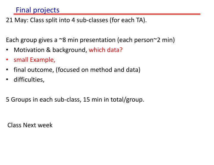
Final projects 21 May: Class split into 4 sub-classes (for each TA). Each group gives a ~8 min presentation (each person~2 min) • Motivation & background, which data? • small Example, • final outcome, (focused on method and data) • difficulties, 5 Groups in each sub-class, 15 min in total/group. Class Next week

Topics: Make sure you only solve a small part 1 Source Localization in an Ocean Waveguide Using Unsupervised ML 3 ML Methods for Ship Detection in Satellite Images 4 Transparent Conductor Prediction 4 Classify ships in San Francisco Bay using Planet satellite imagery 2 Fruit Recognition 3 Bone Age Prediction 1 Facial Expression Classification into Emotions 2 Urban Scene Segmentation for Autonomous Vehicles 1 Face Detection Using Deep Learning 2 Understanding the Amazon Rainforest from Space using NN 4 Mercedez Bench Test Time Estimation 3 Vegetation classification in Hyperspectral Images 4 Threat Detection with CNN 2 Plankton Classification Using ResNet and Inception V3 3 U-net on Biomedical Images 4 Image to Image Transformation using GAN 1 Dog Breed Classification Using CNN 1 Dog Breed Identification 2 Plankton Image Classification 3 Sunspot Detection

��������������� � ����������������������� What is a Graph � ������������������������������������������ • Set of nodes (vertices) � ������������������������������������������������������ • Might have properties associated with them • Set of edges (arcs) each consisting of pair of nodes � ������������������� • Undirected � ������������������� • Directed � �������������������������������������������� • Unweighted or weighted � ����������������������� ��� �� ��� �� �����������������

Road network • Model road system using graph • Nodes where road meet • Edges connections between points • Each edge has a weight Expected time time to get from source node to destination node • Distance along from source node to destination node • • Solve a graph optimization problem • Shortest weighted path between departure and destination node

Trees Undirected Tree Directed Tree Polytree

f = 750 Hz Location 1: Otis Redding - “Hard to handle” 30-microphone array i j Spectral coherence between i and j Location 1: Prince - “Sign o’ the times” (Normalization: |X(f,t)| 2 =1) 6

Trees What would you do tonight? Decide amongst the following: Finish homework • Go to a party • Read a book • Hang out with friends Homework'Deadline' tonight?' Yes ' No ' Do'homework' Party'invitaNon?' Yes ' No ' Do'I'have'friends' Go'to'the'party' Yes ' No ' Hang'out'with' Read'a'book' friends'

Regression Trees (Fig 9.2 in Hastie) R 5 R 2 t 4 X 2 R 3 t 2 R 4 R 1 t 1 t 3 X 1 X 1 X 1 ≤ t 1 | X 2 ≤ t 2 X 1 ≤ t 3 X 2 ≤ t 4 R 1 R 2 R 3 X 2 X 1 R 4 R 5

Details of the tree-building process 1. Divide the predictor space, the set of possible values for X 1 ,X 2 ,...,X p , into J distinct and non-overlapping regions, R 1 , R 2 , . . . , R J . 2. For every observation that falls into the region R j , we make the same prediction, which is simply the mean of the response values for the training observations in R j . The goal is to find boxes R1,...,RJ that minimize the RSS (residual sum square), given by J X X y Rj ) 2 , ( y i − ˆ j =1 i ∈ R j where ! " #$ is the mean response for the training observations within the jth box. X 2 X 1

� Trees (Murphy 16.1) An alternative approach is to dispense with kernels altogether, and try to learn useful features φ ( x ) directly from the input data. That is, we will create what we call an adaptive basis- function model (ABM), which is a model of the form M � f ( x ) = w 0 + w m φ m ( x ) (16.3) m =1 Classification and regression trees We can write the model in the following form M M � � f ( x ) = E [ y | x ] = w m I ( x ∈ R m ) = w m φ ( x ; v m ) (16.4) m =1 m =1 X 2 X 1

Trees (here regression trees) The Hastie book (chapter 8 &9) is easiest to read M � f ( x ) = c m I ( x ∈ R m ) . (9.10) m =1 � # [% " − ' ( ) ] + We use a sum of squares ∑ " ˆ c m = ave( y i | x i ∈ R m ) . (9.11) Define a split: s R 1 ( j, s ) = { X | X j ≤ s } and R 2 ( j, s ) = { X | X j > s } . (9.12) Then we seek the splitting variable j and split point s that solve � ( y i − c 1 ) 2 + min ( y i − c 2 ) 2 � � � min min . (9.13) c 1 c 2 j, s x i ∈ R 1 ( j,s ) x i ∈ R 2 ( j,s ) X 2 X 1

Trees (here classification trees) In a region R m , the proportion of points in class k is 1 X p k ( R m ) = ˆ 1 { y i = k } . n m { x i ∈ R m ≤ } { } ∈ ∈ We then greedily chooses j, s by minimizing the misclassification error ⇣⇥ ⇤⌘ ⇤ ⇥ argmin 1 − ˆ p c 1 ( R 1 ) + 1 − ˆ p c 2 ( R 2 ) j,s Where c 1 is the most common class in R1 (similar for c 2 ) The split in region Rm on requires Nm splits. ● ● ● ● ● ● 0.8 0.8 ● ● ● ● ● ● ● ● ● ● 0.6 0.6 ● ● ● ● x2 x2 ● ● 0.4 0.4 ● ● ● ● ● ● ● ● 0.2 0.2 ● ● ● ● ● ● ● ● 0.0 0.0 ● ● 0.2 0.4 0.6 0.8 1.0 0.2 0.4 0.6 0.8 1.0 x1 x1

Bootstraping The bootstrap is a fundamental resampling tool in statistics. The Idea in the bootstrap is that we can estimate the true F by the so-called empirical distribution Fˆ Given the training data (x i , y i ), i = 1,…n, the empirical distribution function ( 1 if ( x, y ) = ( x i , y i ) for some i � n P ˆ ( X, Y ) = ( x, y ) = F 0 otherwise =>a discrete probability distribution, putting equal weight (1/n) on observed training points A bootstrap sample of size m from the training data is ( x ∗ i , y ∗ i ) , i = 1 , . . . m where each sample is drawn from uniformly at random from the training data with replacement This corresponds exactly to m independent draws from Fˆ. It approximates what we would see if we could sample more data from the true F. We often consider m = n, which is like sampling an entirely new training set. From Ryan Tibshirani

Bagging A single tree has huge variance as a small change in variable can change the tree. The predictive task is greatly simplified. I.e., In classification, we predict the most commonly occurring class . • • In regression, we take the average response value of points in the region. B ootstrap ag gregat ing , or bagging , is a general-purpose procedure for reducing the variance of a statistical learning method; it is particularly useful in decision trees. we generate B bootstrapped training data sets. We train our method on the bth bootstrapped training set to get ! ∗# $ , the prediction at point x. We average all the predictions: B f bag ( x ) = 1 ˆ ˆ X f ∗ b ( x ) . B b =1

Example: bagging Example (from ESL 8.7.1): n = 30 training data points, p = 5 features, and K = 2 classes. No pruning used in growing trees: Bagging helps decrease the misclassification rate of the classifier (evaluated on a large independent test set). Look at orange curve:

Voting probabilities are not estimated class probabilities Suppose that we wanted estimated class probabilities out of our bagging procedure. What about using, for each k = 1 , . . . K : B ( x ) = 1 1 { ˆ p bag X f tree ,b ( x ) = k } ˆ k B b =1 I.e., the proportion of votes that were for class k ? This is generally not a good estimate. Simple example: suppose that the true probability of class 1 given x is 0.75. Suppose also that each of the bagged classifiers ˆ f tree ,b ( x ) correctly predicts the p bag class to be 1. Then ˆ ( x ) = 1 , which is wrong 1 What’s nice about trees is that each tree already gives us a set of p tree ,b predicted class probabilities at x : ˆ ( x ) , k = 1 , . . . K . These k are simply the proportion of points in the appropriate region that are in each class

Alternative form of bagging This suggests an alternative method for bagging. Now given an input x ∈ R p , instead of simply taking the prediction ˆ f tree ,b ( x ) from each tree, we go further and look at its predicted class p tree ,b probabilities ˆ ( x ) , k = 1 , . . . K . We then define the bagging k estimates of class probabilities: B ( x ) = 1 p bag p tree ,b X ˆ ˆ ( x ) k = 1 , . . . K k k B b =1 The final bagged classifier just chooses the class with the highest probability: ˆ p bag f bag ( x ) = argmax ˆ ( x ) k k =1 ,...K This form of bagging is preferred if it is desired to get estimates of the class probabilities. Also, it can sometimes help the overall prediction accuracy …From Ryan Tibshirani

Random Forrest Random forests provide an improvement over bagged trees by way of a small tweak that decorrelates the trees. This reduces the variance when averaging the trees. As in bagging, we build a number of decision trees on bootstrapped training samples. But when building these decision trees, each split is based on a random selection of K predictors. The chosen split candidates from the full set of p predictors. The split can only one of those m predictors