Fictitious Play beats Simplex for fractional packing and covering - PowerPoint PPT Presentation

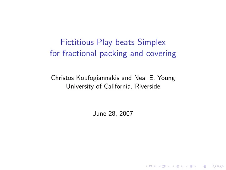
Fictitious Play beats Simplex for fractional packing and covering Christos Koufogiannakis and Neal E. Young University of California, Riverside June 28, 2007

fractional packing and covering Linear programming with non-negative coefficents. Equivalent to solving a zero-sum matrix game A with non-negative coefficients: Theorem (von Neumann’s Min-Max Theorem 1928) A T min max A i x = max min j ˆ x x i x ˆ j x: mixed strategy for min (column) player ˆ x: mixed strategy for max (row) player i: row, j: column ◮ How to compute (1 ± ε )-optimal x and ˆ x quickly? ◮ Simplex algorithm: Ω( n 3 ) time for dense n × n matrix. This talk: O ( n 2 + n log( n ) /ε 2 ) time.

practical performance versus simplex 16384 epsilon = 0.02 epsilon = 0.01 epsilon = 0.005 4096 1024 256 64 speedup: 16 4 1 0.25 0.0625 1024 2048 4096 8192 16384 32768 65536 n = rows, columns

playing a zero-sum game ◮ x = mixed strategy for min ◮ A i x = payoff if max plays row i against mixed strategy x min x : . 5 0 . 5 Ax 1 0 0 . 5 max : A : 1 1 0 . 5 0 1 1 . 5 ← max gets ≤ 5 Min plays x = ( . 5 , 0 , . 5), max gets at most .5 ⇒ game val ≤ . 5.

playing a zero-sum game ◮ x = mixed strategy for min ◮ A i x = payoff if max plays row i against mixed strategy x ◮ ˆ x = mixed strategy for max ◮ A T j ˆ x = payoff if min plays column j against mixed strategy ˆ x min ˆ x . 2 1 0 0 max : . 4 A : 1 1 0 . 4 0 1 1 A T ˆ x : . 6 . 8 . 4 ↑ Max plays ˆ x = ( . 2 , . 4 , . 4), min pays at least .4 ⇒ game val ≥ . 4.

playing a zero-sum game ◮ x = mixed strategy for min ◮ A i x = payoff if max plays row i against mixed strategy x ◮ ˆ x = mixed strategy for max ◮ A T j ˆ x = payoff if min plays column j against mixed strategy ˆ x min x : . 5 0 . 5 ˆ x Ax . 2 1 0 0 . 5 max : . 4 A : 1 1 0 . 5 . 4 0 1 1 . 5 A T ˆ x : . 6 . 8 . 4 Min plays x = ( . 5 , 0 , . 5), max gets at most .5 ⇒ game val ≤ . 5. Max plays ˆ x = ( . 2 , . 4 , . 4), min pays at least .4 ⇒ game val ≥ . 4.

mixed strategies via fictitious play (Brown, Robinson 1951) Repeated play. In each round each player plays single pure strategy, chosen by considering only opponent’s past plays. ◮ x j = #times column j played so far. ◮ ˆ x i = #times row i played so far. ... note | x | = | ˆ x | � = 1 e.g. in 21’st round... min x : 8 1 11 1 0 0 max : 1 1 0 0 1 1 Robinson’s update rule ( x / | x | , ˆ x / | ˆ x | converge to optimal): ◮ Max plays best row against x . ◮ Min plays best col against ˆ x .

mixed strategies via fictitious play (Brown, Robinson 1951) Repeated play. In each round each player plays single pure strategy, chosen by considering only opponent’s past plays. ◮ x j = #times column j played so far. ◮ ˆ x i = #times row i played so far. ... note | x | = | ˆ x | � = 1 e.g. in 21’st round... min x : 8 1 11 Ax 1 0 0 8 max : 1 1 0 9 → 0 1 1 12 ← max plays best row against x Robinson’s update rule ( x / | x | , ˆ x / | ˆ x | converge to optimal): ◮ Max plays best row against x . ◮ Min plays best col against ˆ x .

mixed strategies via fictitious play (Brown, Robinson 1951) Repeated play. In each round each player plays single pure strategy, chosen by considering only opponent’s past plays. ◮ x j = #times column j played so far. ◮ ˆ x i = #times row i played so far. ... note | x | = | ˆ x | � = 1 e.g. in 21’st round... min ↓ x ˆ 1 1 0 0 max : 10 1 1 0 9 0 1 1 A T ˆ x : 11 19 9 ↑ min plays best col against ˆ x Robinson’s update rule ( x / | x | , ˆ x / | ˆ x | converge to optimal): ◮ Max plays best row against x . ◮ Min plays best col against ˆ x .

mixed strategies via fictitious play (Brown, Robinson 1951) Repeated play. In each round each player plays single pure strategy, chosen by considering only opponent’s past plays. ◮ x j = #times column j played so far. ◮ ˆ x i = #times row i played so far. ... note | x | = | ˆ x | � = 1 e.g. in 21’st round... min ↓ x : 8 1 11 x ˆ Ax 1 1 0 0 8 max : 10 1 1 0 9 → 9 0 1 1 12 ← max plays best row against x A T ˆ x : 11 19 9 ↑ min plays best col against ˆ x Robinson’s update rule ( x / | x | , ˆ x / | ˆ x | converge to optimal): ◮ Max plays best row against x . ◮ Min plays best col against ˆ x .

algorithm = smoothed fictitious play random play from exp. distribution (a la Grigoriadis/Khachiyan 1995, expert advice) e.g. in round 201: ε = . 1 min x : 80 10 110 Ax p e 8 1 0 0 80 e 9 max : 1 1 0 90 e 12 0 1 1 120 ◮ max plays random row i from distribution p / | p | where p i = exp( ε A i x ) – concentrated on best columns against x

algorithm = smoothed fictitious play random play from exp. distribution (a la Grigoriadis/Khachiyan 1995, expert advice) e.g. in round 201: ε = . 1 min ˆ x 10 1 0 0 max : 100 1 1 0 90 0 1 1 A T ˆ x : 110 190 90 p : e − 11 e − 19 e − 9 ˆ ◮ min plays random column j from distribution ˆ p / | ˆ p | where ˆ p j = exp( − ε A T j ˆ x ) – concentrated on best rows against ˆ x

algorithm = smoothed fictitious play random play from exp. distribution (a la Grigoriadis/Khachiyan 1995, expert advice) e.g. in round 201: ε = . 1 min x : 80 10 110 ˆ x Ax p e 8 10 1 0 0 80 e 9 max : 100 1 1 0 90 e 12 90 0 1 1 120 A T ˆ x : 110 190 90 p : e − 11 e − 19 e − 9 ˆ ◮ max plays random row i from distribution p / | p | where p i = exp( ε A i x ) – concentrated on best columns against x ◮ min plays random column j from distribution ˆ p / | ˆ p | where ˆ p j = exp( − ε A T j ˆ x ) – concentrated on best rows against ˆ x STOP when max i A i x ≈ ln( n ) /ε 2 or min j A T x ≈ ln( n ) /ε 2 . j ˆ

correctness With high probability, mixed strategies x / | x | for min and ˆ x / | ˆ x | for max are (1 ± O ( ε )) -optimal. Proof. Recall p i = exp( ε A i x ), ˆ p j = exp( − ε A T j ˆ x ), min plays from ˆ p , max from p . | p ′ | × | ˆ p ′ | ≈ 1 + ε p T | p | A ∆ x − ε ˆ p T By algebra: p | A T ∆ˆ x . | p | × | ˆ p | | ˆ ˆ p p By update rule, E [∆ x ] = p | and E [∆ˆ x ] = | ˆ | p | ⇒ expectation of r.h.s. equals 1 (i.e., | p | × | ˆ p | non-increasing) p | = n O (1) ⇒ (w.h.p.) | p | × | ˆ ⇒ max i A i x ≤ min j A T j ˆ x + O (ln( n ) /ε ). Stopping cond’n and weak duality ⇒ (1 ± O ( ε ))-optimal.

implementation in time O ( n 2 + n log( n ) /ε 2 ) ◮ max plays random i from p , where p i = exp( ε A i x ) ◮ min plays random j from ˆ p , where ˆ p j = exp( − ε A T j ˆ x ) STOP when max i A i x ≈ ln( n ) /ε 2 or min j A T x ≈ ln( n ) /ε 2 . j ˆ p (i.e., Ax , A T ˆ Bottleneck is maintaining p , ˆ x ): ∆ x : + 1 ∆ Ax 1 0 0 1 1 0 + 1 0 1 1 + 1 Do work for each increase in a row payoff A i x ... but A i x ≤ ln( n ) /ε 2 , so total work O ( n log( n ) /ε 2 ).

implementation in time O ( n 2 + n log( n ) /ε 2 ) ◮ max plays random i from p , where p i = exp( ε A i x ) ◮ min plays random j from ˆ p , where ˆ p j = exp( − ε A T j ˆ x ) STOP when max i A i x ≈ ln( n ) /ε 2 or min j A T x ≈ ln( n ) /ε 2 . j ˆ p (i.e., Ax , A T ˆ Bottleneck is maintaining p , ˆ x ): ∆ˆ x 1 0 0 1 1 0 + 1 0 1 1 ∆ A T ˆ x : + 1 + 1 Do work for each increase in a row payoff A i x ... or a column payoff A T j ˆ x ... (?!) but A i x ≤ ln( n ) /ε 2 , so total work O ( n log( n ) /ε 2 ).

implementation in time O ( n 2 + n log( n ) /ε 2 ) ◮ max plays random i from p , where p i = exp( ε A i x ) ◮ min plays random j from ˆ p , where ˆ p j = exp( − ε A T j ˆ x ) STOP when max i A i x ≈ ln( n ) /ε 2 or min j A T x ≈ ln( n ) /ε 2 . j ˆ p (i.e., Ax , A T ˆ Bottleneck is maintaining p , ˆ x ): ∆ˆ x 1 0 0 1 1 0 + 1 0 1 1 ∆ A T ˆ x : + 1 + 1 Do work for each increase in a row payoff A i x ... or a column payoff A T j ˆ x ... (?!) but A i x ≤ ln( n ) /ε 2 , so total work O ( n log( n ) /ε 2 ). x ≥ ln( n ) /ε 2 ... ( O ( n 2 ) time) fix: delete column j when A T j ˆ

generalizing to any non-negative matrix A ◮ adapt ideas for width-independence (Garg/K¨ onemann 1998) ◮ random sampling to deal with small A ij ◮ preprocess matrix — approximately sort within each row & column running time for N non-zeros, r rows, c cols: O ( N + ( r + c ) log( N ) /ε 2 ) .

practical performance ◮ first implementation: 10 n 2 + 75 n log( n ) /ε 2 basic op’s ◮ simplex (GLPK): at least 5 n 3 basic op’s for ε ≤ 0 . 05 16384 epsilon = 0.02 epsilon = 0.01 epsilon = 0.005 4096 1024 256 64 speedup: 16 4 1 0.25 0.0625 1024 2048 4096 8192 16384 32768 65536 n = rows, columns

conclusion For dense matrices with thousands of rows and columns, the algorithm finds near-optimal solution much faster than Simplex! open problems: ◮ improve Luby & Nisan’s parallel algorithm (1993) ◮ mixed packing/covering problems ◮ implicitly defined problems (e.g. multicommodity flow) ◮ dynamic problems