February 19 2019 Habitat Suitability Modelling for Protected Corals - PowerPoint PPT Presentation

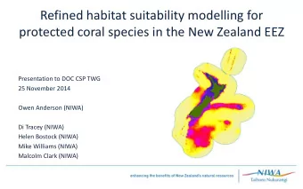
February 19 2019 Habitat Suitability Modelling for Protected Corals

Habitat Suitability Modelling for Protected Corals in New Zealand Waters (POP2018-01) Draft methodology report Owen Anderson Di Tracey Ashley Rowden

Conservation Services Programme Department of Conservation: Project POP2018-01 Objectives • To carry out improved habitat suitability modelling for protected corals in the New Zealand region • To help identify areas of risk from Solenosmilia variabilis reef-like habitat forming scleractinian coral interactions with commercial fishing gear

Rationale • Protected corals frequently occur as bycatch in NZ commercial fisheries (mainly bottom trawl) • To determine the extent of the overlap between fishing and protected coral habitat, first we must determine the spatial extent of each • Habitat Suitability Models – used to explore the relationship between point-sampled species occurrence records and sets of spatially continuous environmental variables • We build on previous studies, incorporating new records, new regional environmental predictor layers from the NZ Earth System Model, and Keratoisis bamboo coral updated modelling approaches • Resulting grids of predicted coral distributions (present and future) can then be used to more precisely define the risk to corals from fishing (and climate change); and inform resource management planning

Habitat suitability modelling Statistical model (including internal validation) Species occurrence records and Map of probability of suitable habitat maps of environmental variables

Environmental predictors New Zealand Earth System Model (NZESM) • Currently under development by NIWA • Incorporates component models of ocean biogeochemistry and other aspects of biology and chemistry to provide a highly complex model of the climate system • This ESM is specifically tuned to the New Zealand region of the Pacific and Southern Oceans • Capable of producing projections for up to 200 years into the future (Williams et al. 2016). Present 2100 AD

Environmental predictors Variable Description Units Reference Seamount Seamount positions in the New Zealand region – Rowden et al. (2008), Mackay (2007) ° Slope Seafloor slope derived from bathymetry CANZ (2008), Hadfield et al. (2002) Dissolved Inorganic Carbon Seafloor DIC concentration mol/m3 NZESM NZESM Sea surface height Sea surface height above geoid m NZESM Bottom temperature In-situ bottom temperature Degrees C NZESM Aragonite concentration Seafloor aragonite concentration mol/m3 NZESM Calcite concentration Seafloor calcite concentration mol/m3 NZESM Nitrate concentration Seafloor dissolved nitrate concentration mol/m3 NZESM Phosphate concentration Seafloor dissolved phosphate concentration mol/m3 NZESM Oxygen concentration Seafloor dissolved oxygen concentration mol/m3 NZESM Chlorophyll concentration Seafloor total chlorophyll mass concentration kg/m3 NZESM Salinity Seafloor salinity g/kg Bostock et al. 2018ab Sediment Percent mud or gravel %

Review of habitat suitability modelling Commonly use sed methods • Generalised Linear Models (GLMs and GAMs) (McCullagh & Nelder 1989, Hastie & Tibshirani 1990) • Maximum Entropy (Maxent) (Phillips et al. 2006) • Random Forests (RF) (Brieman 2001) • Boosted Regression Trees (BRT) (Elith et al. 2008) • Genetic Algorithm for Rule-Set Production (GARP) (Stockwell 1999) • Multivariate Adaptive Regression Splines (MARS) (Friedman 1991) • Ecological Niche Factor Analysis (ENFA) (Hirzel et al. 2002) • Artificial Neural Networks (ANNs) • BIOCLIM (Nix 1986)

New Zealand examples – deep-sea corals Goniocorella dumosa Tracey et al. (2011) • BRT • MBIE, MPI, NIWA G. dumosa

New Zealand examples – deep-sea corals Taiaroa tauhou Compton et al. (2013) • BRT T. tauhou Endemic solitary soft coral • MPI, DOC, LINZ, NIWA

New Zealand examples – deep-sea corals Reef-forming scleractinians Anderson et al. (2016a) • BRT & MaxEnt • SPRFMO region • MBIE, MCI, NIWA

New Zealand examples – deep-sea corals Goniocorella dumosa Anderson et al. (2016b) • BRT & MaxEnt (ensemble) • Precision estimated • NZ region • MBIE, MCI, NIWA

New Zealand examples – deep-sea corals Solenosmilia variabilis Rowden et al. (2017) • BRT & GAM &RF (ensemble) • High resolution (25m 2 ) • Precision estimated • Louisville Seamount Chain • MBIE, MCI, NIWA

New Zealand examples – deep-sea corals Solenosmilia variabilis Anderson et al. (2015) • BRT • Predicting present AND future distributions • DOC, NIWA

Proposed methodology Lessons learned from previous work Recent model validation analyses indicated a general improvement in model reliability over time. The best-performing models were those: • Developed for individual species rather than groups of species • For frequently-recorded species rather than rare species • With a more restricted spatial extent tuned specifically to local environmental conditions • Based on real absence records rather than random background points (pseudo-absence data).

Proposed methodology Coral presence/absence records • Several years of additional records now available, from Observers, research surveys, and overseas institutes • Records from shallower than 200 m will now be included • The focus will be on producing models at the genus or species level • Absence data will be based on research survey stations where the particular taxon was not caught

Proposed methodology Selection of taxa to model • Although models for grouped taxa may be less reliable, this needs to be balanced against limited resources to produce models for many individual species, and also the limited number of individual species with sufficient presence data • Therefore if agreed, some models will be at the genus level and others the species level • Models will be more complex than previous, limiting the total number possible

Proposed methodology Prioritisation of taxa to model Selection of taxa to model Order Taxon Description Number of records Priority (prioritisation) Scleractinia Enallopsammia rostrata Reef-forming coral 130 1 Solenosmilia variabilis Reef-forming coral 311 1 Models will be produced Goniocorella dumosa Reef-forming coral 212 1 Madrepora oculata Reef-forming coral 126 1 for all taxa with priority 1 Alcyonacea Paragorgia arborea (or spp.) Bubblegum coral (tree-like) 98 2 Primnoa spp. Primnoid sea-fans (tree-like) 73 2 Preliminary priorities of 2 Corallium spp Precious coral – 2 Genera combined ( Keratoisis Bamboo corals (tree-like) 241 1 or 3 set for remaining taxa spp. Lepidisis spp.) Antipatharia Bathypathes spp. Black coral (tree-like) 75 1 Leiopathes spp. Black coral (tree-like) 67 3 Anthoathecata Errina spp. Hydrocorals (small, delicate) – 2 Lepidopora or Lepidotheca or – 3 Stylaster (spp.)

Modelling approach Data • Finalise selection of presence and absence data • Finalise selection of environmental variables. A base set of predictors will be chosen for use in all models, modified by specific biological requirements of some taxa. Models (for each method; BRT, RF) • Run separate models by taxon, iteratively as necessary, to derive a residual autocorrelation variable (RAC) to account for spatial autocorrelation • Estimate precision (bootstrapping) • Assess model performance, as a cross-validated AUC value based on subsets of training/test data • Produce final model using the full set of input data. • Use model coefficients to produce two sets of prediction grids; present-day and 2120 AD • Produce ensemble models by averaging predictions from contributing models, weighted by AUC and uncertainty • Produce colour-coded maps of habitat suitability and model uncertainty for each modelled taxon and time period

Overlap between protected corals and bottom trawling Current trawl footprint data obtained from published analysis (Baird & Mules in press) • 5 km x 5km gridded data • Provides both footprint (2D) and aggregated fishing effort (3D) • Covers entire New Zealand EEZ • Recent fishing activity (2008 – 2017) • Depth limited to 200 – 1600 m • Visual matching of coral distributions with footprint/aggregated effort • Overlap statistics calculated • E.g. fraction of cells with high habitat suitability (90% quantile) with high footprint area (>20 km 2 )

Acknowledgements Thanks are extended to CSP, DOC for funding this Project POP2018-01)(NIWA Project Code DOC19301)