Families as Shocks Luis Cubeddu Jos e-V ctor R os-Rull IMF - PowerPoint PPT Presentation
Families as Shocks Luis Cubeddu Jos e-V ctor R os-Rull IMF Penn, CAERP, CEPR August 21, 2002 EEA Meetings, Venezia, August 2002 1. Introduction There is a large literature both in macro and in applied micro (consumption,
Families as Shocks Luis Cubeddu Jos´ e-V´ ıctor R´ ıos-Rull IMF Penn, CAERP, CEPR August 21, 2002 EEA Meetings, Venezia, August 2002
1. Introduction • There is a large literature both in macro and in applied micro (consumption, savings, labor) that considers shocks to earnings or to employment status as the major source of differential outcomes across households (under incomplete insurance markets). • But there are other events in people’s lives that can also be thought as playing a major role in shaping the economic performance of people, and, in particular, their consumption and savings. I am thinking of marital status (another one, health, mostly affects earnings). • Shocks to earnings do not seem to change the total size of wealth much: Aiyagari (1994) measured the size of precautionary savings to be under 10% of savings. More recently, Casta˜ neda et al. (2002) have found that that shocks to earnings increase wealth by 5.5%. EEA Meetings, Venezia, August 2002 1
1. The Plan • Today I want to argue that the type of family structure in which an individual lives and its changes over time play a major role in shaping economic decisions. • I will do it in a very simple manner. Even though we know that people choose which type of family arrangement to live in, I will treat family type as an exogenous event, as a shock, generated by a stochastic process and I will show how dramatically different are the implications of different stochastic processes for the economic outcomes that macroeconomists are interested in, such as the evolution of savings. • For this we need a growth model with agents and households being different things. Let’s build one. EEA Meetings, Venezia, August 2002 2
2. The Model We use an Overlapping Generations Model. Agents are indexed by: • Age: i ∈ { 1 , 2 , · · · , I } . Time ages people: i ′ = i + 1 . • Sex: g ∈ { m, f } , ( g ∗ is spouse’s gender). Sex of agents does not change: g ′ = g . • Marital Status: z ∈ { s o , s w , 1 , 2 , · · · , I } , (Single without and with dependents This we think of a shock: with π i,g ( z ′ | z ) being the and the spouse’s age). probability of moving to state z ′ , conditional on being in state z . • Assets: a ∈ A . These assets are attached to the household and it varies both because of savings and because of changes in the composition of the household. EEA Meetings, Venezia, August 2002 3
2.a Simplest Demographics • Constant population, no early death � π i,g ( z ′ | z ) µ i,g,z µ i +1 ,g,z ′ = z – µ i,g,z : Measure of people of type { i, g, z } . • Consistency of demographic conditions (measure age i males married to age j females equals measure age j females married to age i males). µ i,m,j = µ j,f,i EEA Meetings, Venezia, August 2002 4
2.b Preferences and Endowments �� I � i =1 β i − 1 u i,z ( c ) • Preferences of an age 1 individual. E � � c • Household type affects consumption (equivalence scales): u i,z ( c ) = u . η i,z (no time allocation or fertility decisions). • Labor earnings endowment: ε i,g,z . For most of today’s marital status does not affect earnings: ε i,g,z = ε i,g for all z ∈ Z . 2.c Markets • No insurance for changes in marital status nor life insurance. (perhaps there is a lot of moral hazard). • No borrowing possibilities (not very important). EEA Meetings, Venezia, August 2002 5
2.d Marital Property Status • We assume common property of all household assets, no memory of who brought what to the household. • This is not necessarily the law of all countries but it is the de facto system for most people, those with few assets, or those with small differences in assets at the time of marriage. • An important question is the extent to which property can be protected (e.g. young people save mostly in the form of human capital that is typically non– transferable). EEA Meetings, Venezia, August 2002 6
2.e Single Agent’s Problem: z ∈ { s o , s w } c ≥ 0 ,y ∈A u i,g,z ( c ) + β E { v i +1 ,g,z ′ ( a ′ ) | z } v i,g,z ( a ) = max s.t. c + y = (1 + r ) a + w ε i,g,z if z ′ ∈ { s o , s w } a ′ = y if z ′ ∈ { 1 , .., I } a ′ = y + A z ′ ,g ∗ • A z ′ ,g ∗ : Assets spouse brings into marriage. (Random variable). • Agent must know asset distribution of prospective partners. EEA Meetings, Venezia, August 2002 7
2.f Married Couple’s Problem: z ∈ { 1 , .., I } • We need to specify a bunch of details of how the family is organized and of how the decisions are made. The choices that we made are 1. Spouses are constrained to enjoy equal consumption. 2. Subject to common property regime (assets cannot be traced to its original owner). 3. The household solves a joint maximization problem with weights: ξ i,m,j = 1 − ξ j,f,i . 4. Upon divorce, assets are divided • ψ i,g,j : fraction of assets to { i, g, j } • ψ j,g ∗ ,i : fraction of assets to spouse. • May add to less than 1 because of divorce costs. EEA Meetings, Venezia, August 2002 8
2.g Married Couple’s Problem: z ∈ { 1 , .., I } cont. g ( a ′ g ∗ ( a ′ max u i,g,j ( c ) + β ξ i,g,j E { v i +1 ,g,z ′ g ) | j } + β ξ j,g ∗ ,i E { v j +1 ,g ∗ ,z ′ g ∗ ) | i } c ≥ 0 ,y ∈A c + y = (1 + r ) a + w ( ε i,g,j + ε j,g ∗ ,i ) a ′ g = a ′ • if no divorce: g ∗ = y. a ′ � g = ψ i,g,j y, • if divorce and no remarriage: a ′ g ∗ = ψ j,g ∗ ,i y. a ′ g = ψ i,g,j y + A z ′ g ,g ∗ , � • if divorce and remarriage a ′ g ∗ = ψ j,g ∗ ,i y + A z g ∗ ,g . EEA Meetings, Venezia, August 2002 9
2.h Equilibrium • We look at stationary situations where the key Equilibrium object, φ i,g,z , is a probability measure on assets: • φ i,g,z ( B ) µ i,g,z : Measure of agents type { i, g, z } with assets in B . Equilibrium requires that agents solve their problem given factor prices and distribution of wealth φ , and that there is consistency of wealth distribution and individual behavior: � � π i,g ( z ′ | z ) φ i +1 ,g,z ′ ( B ) = χ a ′ i,g,z ( a ) ∈ B φ i,g,z ( da ) a ∈A z ∈ Z where χ is the indicator function. EEA Meetings, Venezia, August 2002 10
3. A baseline economy without demographic change • No early mortality, no population growth, no productivity growth. • One half of the population starts married to people of their own age. They have an age dependent number of children that peaks at age 43. • The other half starts single, a quarter with and a quarter without dependents. Those that have dependents have one. The lack of change over time makes all singles look in many ways identical. • There is no further demographic change. This is like a standard economy without marital considerations. • Marital status does not affect earnings. • There are economies of scale in consumption. • Calibrated to a wealth to output ratio of 4.15 and NIPA. Interest rate is 2.48%. EEA Meetings, Venezia, August 2002 11
Population Measure (Male, No Change−Baseline) 100 80 Percent 60 40 Married 20 Single w/o Dep Single w/ Dep 0 20 30 40 50 60 70 80 Age EEA Meetings, Venezia, August 2002 12
Earnings (per person) No Change−Baseline 0.4 Married Single Males 0.35 Single Females 0.3 0.25 Earnings 0.2 0.15 0.1 0.05 0 20 30 40 50 60 70 80 Age EEA Meetings, Venezia, August 2002 13
Assets (per person) (Overall, No Change−Baseline) 3 Married All Single Males 2.5 All Single Females 2 Asset 1.5 1 0.5 0 20 30 40 50 60 70 80 Age EEA Meetings, Venezia, August 2002 14
Other economies with changes in marital status • 2. An economy where all people start as singles (half with and half without dependents) and they all marry at age 47 (there is no divorce and the same marriages as in base). • 3. An economy where all people start married and they all divorce. One half ends up with dependents and one half without. Females keep 60% of assets, and males 40%. • 4. An economy where all people alternate, being one period married and one single (again 50% married, 25% singles with and 25% without). • 5. An economy where marital status is i.i.d. • 6. An economy like the U.S. in the nineties. EEA Meetings, Venezia, August 2002 15
Population Structure 2. Late Mar 3. Late Div 1. Base 100 100 100 80 Percent 60 50 50 40 Married 20 Single w/o Dep Single w/ Dep 0 0 0 20 40 60 80 20 40 60 80 20 40 60 80 4. Altern 5. IID 6. 90s 100 100 100 Percent 50 50 50 0 0 0 20 40 60 80 20 40 60 80 20 40 60 80 Age Age Age EEA Meetings, Venezia, August 2002 16
What are their macroeconomic properties? Economy Wealth W/Y r 1. Base 4.15 4.15 2.48% 2. Late Marriage 2.76 3.13 4.73% 3. Late Divorce 5.00 4.65 1.57% 4. Alternation 1.28 1.67 10.1% 5. i.i.d. Marital Status 2.66 3.01 4.95% 6. U.S. in the nineties – 3.24 4.54% • Huge differences in assets holdings. These are general equilibrium effects; partial equilibrium effects are much larger. • Future marriages are serious disincentives to save, especially later in life: the rate of return is negative. • Late divorce are incentives to save. Females’ lower earnings and higher share of assets makes them want to save (equal weights in decisions). • Turnover lowers savings but not always. The effects are big. EEA Meetings, Venezia, August 2002 17
Recommend
More recommend
Explore More Topics
Stay informed with curated content and fresh updates.
