Factorizing a string into squares in linear time Yoshiaki Matsuoka, - PowerPoint PPT Presentation
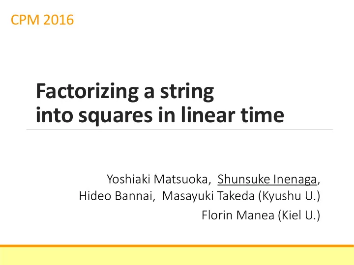
CPM 2016 Factorizing a string into squares in linear time Yoshiaki Matsuoka, Shunsuke Inenaga, Hideo Bannai, Masayuki Takeda (Kyushu U.) Florin Manea (Kiel U.) From string to squares? In this presentation, I talk about decomposition of a
CPM 2016 Factorizing a string into squares in linear time Yoshiaki Matsuoka, Shunsuke Inenaga, Hideo Bannai, Masayuki Takeda (Kyushu U.) Florin Manea (Kiel U.)
From string to squares? In this presentation, I talk about decomposition of a string into squares .
Squares (as strings!) “Our square” is a string of form xx . aabaab aba bababab aba babaababa
Primitively rooted squares A square xx is called a primitively rooted square if its root x is primitive (i.e., x ≠ y k for any string y and integer k ). aabaab : primitively rooted square aba bababab : not primitively rooted square aba babaababa : : primitively rooted square
Our problem Determine whether a given string can be factorized into a sequence of squares. If the answer is yes, then compute one of such factorizations. E.g.) aabaabaaaaaa → Yes ◦ ( aabaab , aaaaaa ), ◦ ( aabaab , aaaa , aa ), ◦ ( aa , baabaa , aa , aa ) , and so on. aabaabbbab → No 5
Previous work Times for computing square factorization [Dumitran et al., 2015] A sq. factor. O ( n log n ) n is the length of the input string. 6
Previous work Times for computing square factorization [Dumitran et al., 2015] A sq. factor. O ( n log n ) Largest sq. O ( n log n ) factor. n is the length of the input string. 7
Our contribution Times for computing square factorization [Dumitran et al., 2015] Our solutions A sq. factor. O ( n log n ) O ( n ) Largest sq. O ( n + ( n log 2 n ) / ω ) O ( n log n ) factor. Smallest sq. - O ( n log n ) factor. n is the length of the input string. Our results for arbitrary/largest square factorizations are valid on word RAM with word size ω = Ω(log n ) . 8
Our contribution Times for computing square factorization [Dumitran et al., 2015] Our solutions A sq. factor. O ( n log n ) O ( n ) Largest sq. O ( n + ( n log 2 n ) / ω ) O ( n log n ) factor. Smallest sq. - O ( n log n ) factor. n is the length of the input string. Our results for arbitrary/largest square factorizations are valid on word RAM with word size ω = Ω(log n ) . 9
Simple observation Every square is of even length. Thus, if string w has a square factorization, then w also has a square factorization which consists only of primitively rooted squares . E.g.) aaaaaa|abababab aa|aa|aa|abab|abab
# of primitively rooted squares Any string of length n contains O ( n log n ) primitively rooted squares [Crochemore & Rytter, 1995]. The simple observation + the above lemma lead to a natural DP approach which computes a square factorization in O ( n log n ) time.
Dumitran et al.’s algorithm Consider the following DAG G for string w : There are n +1 nodes. There is a directed edge ( e +1, b ) in G . ⟺ Substring w [ b .. e ] is a primitively rooted square. a a b a a b a a a a
Dumitran et al.’s algorithm Consider the following DAG G for string w : There are n +1 nodes. There is a directed edge ( e +1, b ) in G . ⟺ Substring w [ b .. e ] is a primitively rooted square. a a b a a b a a a a
Dumitran et al.’s algorithm DAG G has a path from the rightmost node to the leftmost node. ⟺ There is a square factorization of w . a a b a a b a a a a
Dumitran et al.’s algorithm a a b a a b a a a a 0 0 0 0 0 0 0 0 0 0 1 The rightmost node is associated with a 1 . Initially, all the other nodes are associated with 0 ’s.
Dumitran et al.’s algorithm a a b a a b a a a a 0 0 0 0 0 0 0 0 0 0 1 We process each node from right to left. Each node v gets a 1 iff there is an in- coming edge to v from a node that is associated with a 1 .
Dumitran et al.’s algorithm a a b a a b a a a a 0 0 0 0 0 0 0 0 0 0 1 We process each node from right to left. Each node v gets a 1 iff there is an in- coming edge to v from a node that is associated with a 1 .
Dumitran et al.’s algorithm a a b a a b a a a a 0 0 0 0 0 0 0 0 0 0 1 1 We process each node from right to left. Each node v gets a 1 iff there is an in- coming edge to v from a node that is associated with a 1 .
Dumitran et al.’s algorithm a a b a a b a a a a 0 0 0 0 0 0 0 0 1 0 0 1 We process each node from right to left. Each node v gets a 1 iff there is an in- coming edge to v from a node that is associated with a 1 .
Dumitran et al.’s algorithm a a b a a b a a a a 0 0 0 0 0 0 0 0 1 1 0 0 1 We process each node from right to left. Each node v gets a 1 iff there is an in- coming edge to v from a node that is associated with a 1 .
Dumitran et al.’s algorithm a a b a a b a a a a 1 0 1 0 0 0 1 0 1 0 0 1 Finally, there is a square factorization of the string iff the leftmost node is associated with a 1 .
Dumitran et al.’s algorithm a a b a a b a a a a 1 0 1 0 0 0 1 0 1 0 0 1 A path from the rightmost node to the leftmost node corresponds to a square factorization.
Dumitran et al.’s algorithm a a b a a b a a a a 1 0 1 0 0 0 1 0 1 0 0 1 Another path from the rightmost node to the leftmost node corresponds to another square factorization.
Dumitran et al.’s algorithm a a b a a b a a a a 1 0 1 0 0 0 1 0 1 0 0 1 Clearly, the number of edges in this DAG is equal to the number of primitively rooted squares in the string, which is O ( n log n ) . Hence, their algorithm takes O ( n log n ) time.
Ideas of our O ( n ) -time algorithm We accelerate Dumitran et al.’s algorithm by a mixed use of runs uns (maximal repetitions in the string); bit t para rallelism (performing some DP computation in a batch).
Runs A triple ( p , b , e ) of integers is said to be a run of a string w if The substring w [ b .. e ] is a repetition with the smallest period p (i.e., 2 p ≤ e − s +1 ), and The repetition is non-extensible to left nor right with the same period p . (3, 1, 8) a a b a a b a a a a (1, 1, 2) (1, 4, 5) (1, 7, 10)
Long and short period runs Let w be the machine word size. A run ( p , b , e ) in a string is called a long period run ( LPR ) if 2 p ≥ w ; a short period run ( SPR ) if 2 p < w . E.g.) For w = 4 LPR (3, 1, 8) a a b a a b a a a a SPR (1, 1, 2) SPR (1, 4, 5) SPR (1, 7, 10)
Long edges Edges that correspond to long period runs are called long edges. LPR (3, 1, 8) a a b a a b a a a a
Short edges Edges that correspond to short period runs are called short edges. SPR (1, 1, 2) SPR (1, 4, 5) SPR (1, 7, 10) a a b a a b a a a a
How to process long edges We partition the nodes into blocks of length w each. Processing this block … … … … 1 1 0 0 0 0 1 0 0 1 1 1
How to process long edges Since the long edges that correspond to the same LPR have the same length and are consecutive, we can process w of them in a batch, by performing a bit-wise OR. Long edges corresponding to the same LPR Processing this block … … … … 1 0 0 1 1 1 1 1 0 0 0 0 1 0 0 1 1 1 bit-wise OR ※ Our algorithm does NOT create edges explicitly.
How to process long edges Since the long edges that correspond to the same LPR have the same length and are consecutive, we can process w of them in a batch, by performing a bit-wise OR. Long edges corresponding to the same LPR Processing this block … … … … 1 1 0 1 1 1 1 0 0 1 1 1 bit-wise OR ※ Our algorithm does NOT create edges explicitly.
Time cost for long edges We can process at most w long edges in a batch in O (1) time, hence we can process all long edges in O (( n log n )/ w ) time. An O ( n + # LPR) -time preprocessing allows us to perform the these operations without constructing long edges explicitly. Thus we need O ( n + #LPR + ( n log n )/ w ) total time for long edges.
How to process short edges Every short edge is shorter than w . Hence, for each node i , it is enough to consider at most w in-coming short edges. i + ω i … … 0 0 0 1 0 1 0 ※ Our algorithm does NOT create edges explicitly.
How to process short edges To process these short edges in a batch, we use a bit mask B i indicating if each node has a short edge to node i . i + ω i … … 0 0 0 1 0 1 0 0 1 0 0 1 1 B i = ※ Our algorithm does NOT create edges explicitly.
How to process short edges To process these short edges in a batch, we use a bit mask B i indicating if each node has a short edge to node i . i + ω i … … 0 0 0 1 0 1 0 bitwise AND 0 1 0 0 1 1 B i = = bitwise AND 0 0 0 0 1 0 ※ Our algorithm does NOT create edges explicitly.
How to process short edges If there is a 1 in the resulting bit string, then node i gets a 1 . i + ω i … … 0 0 0 1 0 1 0 bitwise AND 0 1 0 0 1 1 B i = = bitwise AND 0 0 0 0 1 0 ※ Our algorithm does NOT create edges explicitly.
Recommend
More recommend
Explore More Topics
Stay informed with curated content and fresh updates.
