Exponential Random Graph Models for (Social) Network Data Analysis - - PowerPoint PPT Presentation

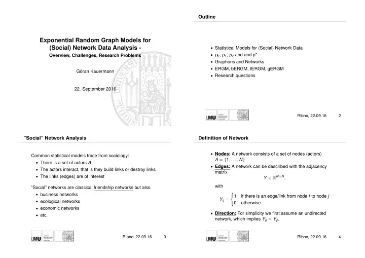
Outline Exponential Random Graph Models for (Social) Network Data Analysis - • Statistical Models for (Social) Network Data • p 0 , p 1 , p 2 and and p* Overview, Challenges, Research Problems • Graphons and Networks • ERGM, bERGM, tERGM, gERGM G¨ oran Kauermann • Research questions 22. September 2016 Ribno, 22.09.16 2 ”Social” Network Analysis Definition of Network • Nodes: A network consists of a set of nodes (actors) Common statistical models trace from sociology: A = { 1 , . . . , N } • There is a set of actors A • Edges: A network can be described with the adjacency • The actors interact, that is they build links or destroy links matrix • The links (edges) are of interest Y ∈ R N ⇥ N , with ”Social” networks are classical friendship networks but also ( • business networks 1 if there is an edge/link from node i to node j Y ij = • ecological networks 0 otherwise • economic networks • Direction: For simplicity we first assume an undirected • etc. network, which implies Y ij = Y ji . Ribno, 22.09.16 3 Ribno, 22.09.16 4

”Classical” Network Models: The p 0 Model ”Classical” Network Models: The p 1 Model • p 1 Model (Holland and Leinhardt, 1981) ✓ ◆ • Erd¨ os-Renyi Model (1959) P ( Y ij = 1 ) � � = α i + α j + z t logit P ( Y ij = 1 ) = log ij β 1 − P ( Y ij = 1 ) P ( Y ij = 1 ) = π • The p 1 Model assumes conditional independence of the • Independence of edges (and nodes) edges • Parameter π gives the average density • Node (actor) specific effects α i , i = 1 , . . . , N • Very simplistic model, may serve as intercept or null model • Edge (pair) specific covariate effects β • The model is a standard logit model • Can be fitted with standard software Ribno, 22.09.16 5 Ribno, 22.09.16 6 ”Classical” Network Models: The p 2 Model ”Classical” Network Models: The p* Model • p 2 Model (Duijn et al., 2004 and Zijlstra et al., 2006) • p* model or better known as Exponential Random Graph � � = φ i + φ j + z t Model (ERGM) (Frank and Strauss, 1986) logit P ( Y ij = 1 | Φ ) (1) ij β , Φ = ( φ 1 , . . . , φ n ) t ∼ N ( 0 , σ 2 � � φ I n ) θ T s ( y ) P ( Y = y | θ ) = exp κ ( θ ) • The model reduces the number of parameters for large networks • κ ( θ ) is a normalizing constant • The p 2 model induces nodal heterogeneity • s ( y ) is a vector of so-called network statistics • The modal results in a standard generalized linear mixed model (GLMM) • The model is an exponential family • Can be fitted with standard software Ribno, 22.09.16 7 Ribno, 22.09.16 8

Features of ERGM A First Comparison Modelling Unobserved Network Usability in Estimation • Unlike in the p 1 and p 2 model the edge Y ij depends on the Flexibility Modal Dependence Large rest of the network Y \ Y ij Heterogeneity networks (N → ∞ ) • Edge between node i and j depends on the ”individual” network of the two nodes p0 - - - X X • Conditional model p1 only parametric - X X covariates logit [ P ( Y ij = 1 | Y \{ Y ij } , θ )] = θ T [ s ( y ij = 1 , Y \{ Y ij } ) − s ( y ij = 0 , Y \{ Y ij } )] p2 only random - X X | {z } covariates := ∆ s ij ( y ) p* network and - X - - where ∆ s ij ( y ) denotes the vector of change statistics covariates Ribno, 22.09.16 9 Ribno, 22.09.16 10 ERGM: Estimation Problem (1) Estimation Problem (2) • Pseudo likelihood (Ikeda and Strauss, 1990): One assume independence of the edges, i.e. • The normalization constant κ ( θ ) is numerically infeasible, logit P ( Y ij = 1 | Y \{ Y ij } ) = logit P ( Y ij = 1 ) = ∆ s ij ( y ) θ since X κ ( θ ) = exp ( s ( y ) θ ) y 2 Y where Y = set of possible networks with N nodes • |Y| = 2 N ( N + 1 ) / 2 , for N = 10 ⇒ 3 · 10 13 networks • Estimation requires numerical simulation tools Ribno, 22.09.16 11 Ribno, 22.09.16 12

Estimation Problem (2) Estimation Problem (2) • Pseudo likelihood (Ikeda and Strauss, 1990): • Pseudo likelihood (Ikeda and Strauss, 1990): One assume independence of the edges, i.e. One assume independence of the edges, i.e. logit P ( Y ij = 1 | Y \{ Y ij } ) = logit P ( Y ij = 1 ) = ∆ s ij ( y ) θ logit P ( Y ij = 1 | Y \{ Y ij } ) = logit P ( Y ij = 1 ) = ∆ s ij ( y ) θ ⇒ Estimation is simple, but estimates are biased and ⇒ Estimation is simple, but estimates are biased and inference is invalid inference is invalid • Simulation based (Hunter and Handcock, 2006): We approximate X exp ( θ s ( y ⇤ )) κ ( θ ) ≈ s ( y ∗ ) where y ⇤ are random draws from the ERGM Ribno, 22.09.16 13 Ribno, 22.09.16 14 Estimation Problem (2) Estimation of ERGM (3) • Pseudo likelihood (Ikeda and Strauss, 1990): One assume independence of the edges, i.e. • Fully Bayesian Estimation (Caimo and Friel, 2011): logit P ( Y ij = 1 | Y \{ Y ij } ) = logit P ( Y ij = 1 ) = ∆ s ij ( y ) θ We are interested in the posterior distribution ⇒ Estimation is simple, but estimates are biased and π ( θ | y ) ∝ π ( y | θ ) π ( θ ) , inference is invalid • Simulation based (Hunter and Handcock, 2006): with π ( θ ) as prior distribution on θ . We approximate X exp ( θ s ( y ⇤ )) κ ( θ ) ≈ s ( y ∗ ) where y ⇤ are random draws from the ERGM ⇒ Estimation is unstable and numerically demanding Ribno, 22.09.16 15 Ribno, 22.09.16 16

Estimation of ERGM (3) Estimation of ERGM (4) Solution: Bergm: Exchange algorithm - We sample from an augmented distribution • Fully Bayesian Estimation (Caimo and Friel, 2011): π ( θ 0 , y 0 , θ | y ) ∝ π ( y | θ ) π ( θ ) h ( θ 0 | θ ) π ( y 0 | θ 0 ) . We are interested in the posterior distribution π ( θ | y ) ∝ π ( y | θ ) π ( θ ) , 1 Gibbs update of ( θ 0 , y 0 ) : with π ( θ ) as prior distribution on θ . i. Draw θ 0 ∼ h ( ·| θ ) . ii. Draw y 0 ∼ π ( ·| θ 0 ) . Problem: This posterior is “doubly-intractable”, because 2 Propose the exchange move from θ to θ 0 with probability neither the normalisation constant of π ( y | θ ) nor of π ( θ | y ) is known. ✓ ◆ 1 , q ( y 0 | θ ) π ( θ 0 ) h ( θ | θ 0 ) q ( y | θ 0 ) q ( y | θ ) π ( θ ) h ( θ 0 | θ ) q ( y 0 | θ 0 ) × κ ( θ 0 ) κ ( θ ) α = min . κ ( θ ) κ ( θ 0 ) Ribno, 22.09.16 17 Ribno, 22.09.16 18 Problems in ERGM Extension: Heterogeneity of Actors • ERGMs are notoriously unstable, i.e. the reasonable We have extended the model to allow for heterogeneous actors parameter space (Thiemichen et al., 2016) Θ 0 = { θ : density(Network) is bounded away form 0 and 1 } ⇥ � ⇤ = θ T ∆ s ij ( y ) + φ i + φ j , logit P ( Y ij = 1 � Y \ { Y ij } , θ , φ ) is getting smaller for N → ∞ with φ i ∼ N ( µ φ , σ 2 φ ) , for i = 1 , ..., n . • As a consequence: simulated networks are either full or empty This leads to the entire model • Bayesian approaches circumvent this problem for the price � � θ T s ( y ) + φ T t ( y ) P ( Y = y | θ , φ ) = exp of heavy computation (i.e. low acceptance rate) , κ ( θ , φ ) Two reasons for instability: ! 1 The models assume that the nodes are homogeneous P y 1 j , P y 2 j , . . . , P where t ( y ) = y nj . 2 Network statistics are unstable , i.e. there is an avalanche j 6 = 1 j 6 = 2 j 6 = n effect. Ribno, 22.09.16 19 Ribno, 22.09.16 20

Fully Bayesian Inference Instable Network Statistics We are interested in • Network statistics ought to be s ( y ) = 0 ( N 2 ) π ( θ , φ | y ) ∝ π ( y | θ , φ ) π ( θ ) π ( φ ) . (Schweinberger, 2011) This can be estimated with the exchange algorithm from above • two-star, triangle, etc. are all unstable (Bergm). • Geometrically weighted statistics (Snijders et al., 2006), We are additionally interested in σ 2 φ , i.e. e.g. • geometrically weighted degree (gwd) π ( θ , φ , σ 2 φ | y ) ∝ π ( y | θ , φ ) π ( θ ) π ( φ ) π ( σ 2 φ ) . • geometrically weighted edgewise shared parameter (gwesp) with π ( σ 2 φ ) as inverse gamma. • Smooth statistics (Talk on Friday, Thiemichen) Problem: Estimation is numerically very demanding Ribno, 22.09.16 21 Ribno, 22.09.16 22 Stable Network Statistics What happens if Networks are Large? Snijders, Pattison, Robins and Handcock (2006) proposed new geometrically downweigted network statistics which behave stable . • Geometrically weighted degree (gwd) • ”Classical” models hardly scale to large networks with • Geometrically weighted edgewise shared partners (gwesp) 1000 or more actors N � 2 • Estimation becomes computationally too demanding X { 1 − q l ) ESP l ( y ) s ( y , q ) = • Homogeneity of actors is questionalble l = 1 • Clustering (grouping) of actors seems more useful where q is a decay parameter and ESP l ( y ) is the number of edges with l joint partners. • Note: The gwesp statistics is edge based and not node based . • Note: Interpretation gets clumsy . Ribno, 22.09.16 23 Ribno, 22.09.16 24