Exploration of Lossy Compression for Application- level - PowerPoint PPT Presentation

LLNL-PRES-670952 � Exploration of Lossy Compression for Application- level Checkpoint/Restart � Naoto Sasaki 1 , Kento Sato 3 , Toshio Endo 1,2 , Satoshi Matsuoka 1,2 1 Tokyo institute of technology 2 Global Scientific Information and Computing Center 3 Lawrence Livermore National Laboratory

LLNL-PRES-670952 � Needs for Fault Tolerance � The scale of HPC systems are exponentially growing • exa-scale supercomputers in about 2020 • The failure rate increases as systems size grows Applications’ users want to continue its computation even on a failure Checkpoint/Restart technique is widely used as fault tolerant function • But this technique has problems � �

LLNL-PRES-670952 � Needs for Reduction in Checkpoint Time � On TSUBAME2.5 Checkpoint/Restart Memory capacity � about 116TB I/O throughput � about 8GB/s → Data of memory is stored in the disk ↓ → High I/O cost Checkpoint time � about 4 hours � MTBF(Mean Time Between Failure) is reduced by expansion in the scale of HPC systems • MTBF is projected to shrink to over 30min in 2020 [ � 1] If MTBF < Checkpoint time an application may not be able to run � ��������������� ↓ Needs for reduction in checkpoint time ! � Applications’ users need to reduce checkpoint time � 1 : Peter Kogge, Editor & Study Lead (2008) � ExaScale Computing Study: Technology Challenges in Achieving ExaScale Systems �

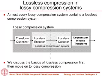
LLNL-PRES-670952 � To Reduce Checkpoint Time � There are techniques to reduce checkpoint size • Compression • Incremental checkpointing • This stores only differences with the last checkpoint Compression can be combined with incremental checkpointing • In addition, the effect of incremental checkpointing may be limited in scientific applications We focus on compression for checkpoint image data �

LLNL-PRES-670952 � Lossless and Lossy Compression � gzip, bzip2, etc. � jpeg, mp4, etc. � Features of lossless Features of lossy • � o data loss • High compression rate • Low compression rate without bias • Error �� are introduced • Scientific data has a randomness � 100 90 If we apply lossless 80 Compression rate [%] compression to floating point 70 arrays, the compression rate 60 50 is limited � 40 30 20 10 We focus on lossy compression � 0 original gzip ��

LLNL-PRES-670952 � Discussion on Errors Introduced by Lossy Methods � Errors may be acceptable if we examine processes for developing real scientific applications • Scientific model and sensors also introduce errors • � e need to investigate whether the errors are acceptable 1/100 � 1/7 � original 14.7MB � gzip 2.19MB � jpeg2000 0.153MB (citation of images : http://svs.gsfc.nasa.gov/vis/a000000/a002400/a002478/) � Don’t apply lossy compression to data that must not have an error (e.g. pointer) We apply lossy compression to checkpoint data • The calculation continues with data including errors ��

LLNL-PRES-670952 � Outline of Our Study � Purpose • To reduce checkpoint time, lossy compression is applied to checkpoint data then checkpoint size is reduced Proposed Approach 1. We apply wavelet transformation, quantization and encoding to a target data, then store the data in a recoverable format 2. We apply gzip to the recoverable format data Contribution • We apply our approach to real climate application, NICAM, then overall checkpoint time included compression time is reduced by 81% with 1.2% relative error on average in particular situation ��

LLNL-PRES-670952 � Assumption for Our Approach � We assume application � level checkpoint • We utilize that difference between neighbor values • Target data are an arrays of physical quantities • We target 1,2 or 3D mesh data represented by floating point arrays There are data to which must not be applied our approach because errors are introduced • Data structure including pointers (e.g. tree) Users specify a range of data to which are applied our approach ��

LLNL-PRES-670952 � Motivation of Wavelet Transformation � Lossless compression is effective in data that have redundancy • Scientific data has a randomness � • We need to make redundancy in the scientific data To make much redundancy and make errors small … • The target data should have dense and small values The scientific data does not spatially changed much To make good use of this feature … � We focus on wavelet transformation � ��

LLNL-PRES-670952 � About Wavelet Transformation � Wavelet transformation is a technique of frequency analysis We suspect that compression that uses wavelet transformation is efficient in applications that uses physical quantities (e.g. pressure, temperature) � citation of images �� http://www.thepolygoners.com/tutorials/dwavelet/DWTTut.html � Multiple resolution analysis is effective in compression • JPEG2000 uses this technique • It is known that this technique is effective in smooth data • This “ smooth ” means the difference between neighbor values is small � Wavelet transformation itself is NOT compression method, ��� but we use � t for preprocessing

LLNL-PRES-670952 � Proposal Approach � Lossy Compression Based On Wavelet � Original checkpoint data (Floating point array) 1. Wavelet transformation Low-frequency band High-frequency band array array 2. Quantization average High-frequency band array bitmap array 3. Encoding High-frequency band array 4. Formatting average bitmap � Low and high-frequency band arrays array 5. Applying gzip ��� Compressed data

LLNL-PRES-670952 � Wavelet Transformation � Original checkpoint data (Floating point array) 1. Wavelet transformation Low-frequency band High-frequency band array array 2. Quantization average High-frequency band array bitmap array 3. Encoding High-frequency band array 4. Formatting average bitmap � Low and high-frequency band arrays array 5. Applying gzip ��� Compressed data

LLNL-PRES-670952 � 1D Wavelet Transformation in Our Approach � We use average of two neighbor values and difference between two neighbor values � value � Original 1D array � Wavelet index � transformation average � value � Transformed array � difference � High-frequency � Low-frequency � In high-frequency band, most of values are close to zero ��� → We expect that an introduced error is small even if the precision of values in high-frequency band region is dropped �

LLNL-PRES-670952 � Multi-dimensional Wavelet Transformation � Low- High- frequency frequency � In multi-dimensional array, we apply 1D wavelet transformation to each dimension 1D wavelet In case of 2D array • # of low … 1 1D wavelet � • # of high … 3 1 low-frequency In case of 3D array band � • # of low … 1 • # of high … 7 3 high-frequency band � Fig : an example of wavelet transformation for ��� a 2D array �

LLNL-PRES-670952 � Quantization � Original checkpoint data (Floating point array) 1. Wavelet transformation Low-frequency band High-frequency band array array 2. Quantization average High-frequency band array bitmap array 3. Encoding High-frequency band array 4. Formatting average bitmap � Low and high-frequency band arrays array 5. Applying gzip ��� Compressed data

LLNL-PRES-670952 � Simple Quantization � 1. Divide high-frequency band values into n partitions • This n is called the number of division Introduce 2. Replace all values of each partition with an average of an error � the corresponding partition Introduce Introduce an error � an error � n = 4 Calculate an average � Calculate an average � value � value � Focus on Replace � high-frequency band � ��� index � index �

LLNL-PRES-670952 � Problems of Simple Quantization � Simple quantization introduces large errors n = 4 n = 4 Distribution of high-frequency band Frequency average [0] average [2] average [1] average [3] -3 -2.5 -2 -1.5 -1 -0.5 0 0.5 1 1.5 2 2.5 3 3.5 -3 -2.5 -2 -1.5 -1 -0.5 0 0.5 1 1.5 2 2.5 3 3.5 -3 -2.5 -2 -1.5 -1 -0.5 0 0.5 1 1.5 2 2.5 3 3.5 4 4 4 Values in high-frequency band Values in high-frequency band Values in high-frequency band Make histogram � ��� High-frequency band �

LLNL-PRES-670952 � To reduce Errors � Target data is expected to be smooth • Most of values in high-frequency band are close to zero • These make a “ spike” in the distribution To reduce an error, we apply the quantization to the “ spike” parts only • An impact on compression rate is low because the spike parts consist of most of values in high-frequency band Apply quantization to this “spike” part only � No quantization � No ��� quantization � -3 -2.5 -2 -1.5 -1 -0.5 0 0.5 1 1.5 2 2.5 3 3.5 4

LLNL-PRES-670952 � Proposed Quantization � This method is improved version of simple one n = 4 d = 10 average [1] average [2] average [3] average [0] N total d -3 -2.5 -2 -1.5 -1 -0.5 0 0.5 1 1.5 2 2.5 3 3.5 -3 -2.5 -2 -1.5 -1 -0.5 0 0.5 1 1.5 2 2.5 3 3.5 4 -3 -2.5 -2 -1.5 -1 -0.5 0 0.5 1 1.5 2 2.5 3 3.5 4 4 Values in high-frequency band Values in high-frequency band Values in high-frequency band Make histogram � Red elements belong to “ spike ” parts High-frequency band � 0 1 1 1 1 1 1 0 ��� bitmap �