Expected Residual Life time and Years of Life Lost Bendix - PDF document
Expected Residual Life time and Years of Life Lost Bendix Carstensen Steno Diabetes Center Copenhagen, Denmark & Dept. of Biostatistics, University of Copenhagen VicBiostats, Melbourne, 23 February 2017 http://BendixCarstensen.com 1/ 41
Expected Residual Life time and Years of Life Lost Bendix Carstensen Steno Diabetes Center Copenhagen, Denmark & Dept. of Biostatistics, University of Copenhagen VicBiostats, Melbourne, 23 February 2017 http://BendixCarstensen.com 1/ 41 Life lost to disease ◮ Persons with disease live shorter than persons without ◮ The difference is the life lost to disease — years of life lost ◮ Possibly depends on: ◮ sex ◮ age ◮ duration of disease ◮ definition of persons with/out disease ◮ Conditional or population averaged? ◮ . . . the latter gives a seductively comfortable single number ◮ . . . the former confusingly relevant insights 2/ 41 Expected life time — the formals: . . . the age at death integrated w.r.t. the distribution of age at death: � ∞ EL = a f ( a ) d a 0 The relation between the density f and the survival function S is f ( a ) = − S ′ ( a ) , so integration by parts gives: � ∞ � ∞ � ∞ � − S ′ ( a ) � � EL = a d a = − aS ( a ) 0 + S ( a ) d a 0 0 The first term is 0 so: � ∞ EL = S ( a ) d a 0 3/ 41
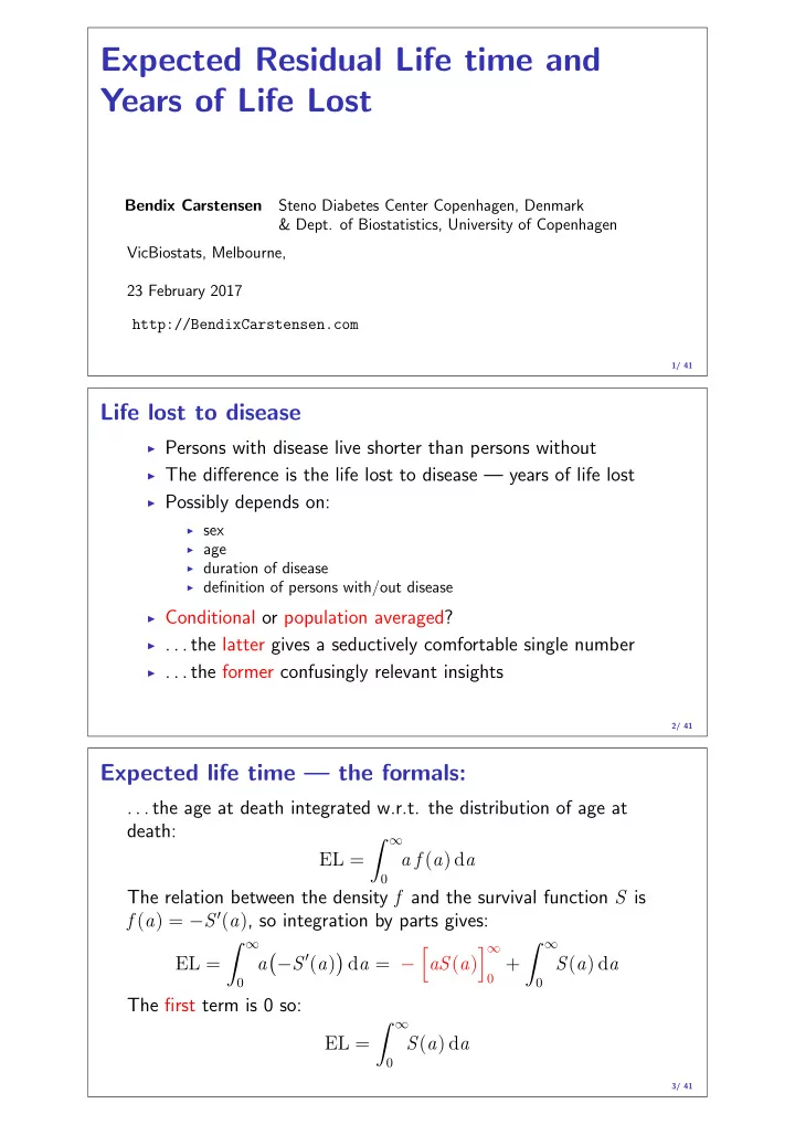
Expected life time illustrated ◮ Take, say 200, persons ◮ follow till all are dead ◮ compute the mean age at death (life time) ◮ — that is the life expectancy (at birth) 4/ 41 0 20 40 60 80 100 Age 5/ 41 0 20 40 60 80 100 Age 6/ 41
Expected life time and years lost ◮ ERL ( E xpected R esidual L ifetime): Area under the survival curve ◮ YLL ( Y ears of L ife L ost) (to diabetes, say): ERL pop − ERL DM ◮ difference between areas under the survival curves ◮ ⇒ area between the curves ◮ . . . all the way till all are dead 7/ 41 Wikipedia: PYLL P otential Y ears of L ife L ost ◮ Fix a threshold, T , (the population EL , or say 75 ) ◮ A person dead in age a < T contributes T − a ◮ A person dead in age a > T contributes 0 . . . seems to assume that the expected age at death is T regardless of attained age ? 8/ 41 WHO — Years of Life Lost Rationale for use Years of life are lost (YLL) take into account the age at which deaths occur by giving greater weight to deaths at younger age and lower weight to deaths at older age. The years of life lost (percentage of total) indicator measures the YLL due to a cause as a proportion of the total YLL lost in the population due to premature mortality. Definition YLL are calculated from the number of deaths multiplied by a standard life expectancy at the age at which death occurs. The standard life expectancy used for YLL at each age is the same for deaths in all regions of the world (. . . ) www.who.int/whosis/whostat2006YearsOfLifeLost.pdf ⇒ a person dying in age a contributes ERL( a ) . . . 9/ 41
Comparing men and women ◮ When a man dies age a , say, ◮ YLL is ERL w ( a ) > 0 ◮ — the expected residual life time of a woman aged a . ◮ When a woman dies age a , say, ◮ YLL is ERL m ( a ) > 0 ◮ — the expected residual life time of a man aged a . ◮ . . . so both sexes lose years relative to the other ! 10/ 41 Healthy lifestyle and excercise. . . ◮ Any one who dies before age 75 (PYLL) ◮ Any one who dies (WHO YLL) ◮ . . . contribute a positive number to YLL ◮ ⇒ any subgroup of the population have positive years of life lost when compared to the general population! ◮ . . . well, indeed compared to any population (men vs. women) ◮ No shortcuts: ◮ no unfounded algorithms ◮ the YLL is a difference of expectations ◮ use a statistical model (specify f ( a ) , that is) ◮ diabetes in Denmark as an example 11/ 41 How the world looks λ (a) Well Well DM DM µ W (a) µ DM (a,d) Dead(DM) Dead(DM) Dead Dead 12/ 41
Comparing DM and well � ∞ YLL = S W ( a ) − S D ( a ) d a 0 the conditional YLL given attained age A , just use: S W ( a | A ) = S W ( a ) / S W ( A ) , S D ( a | A ) = S D ( a ) / S D ( A ) The survival functions we need are: � a � a � � � � S W ( a ) = exp − µ W ( u ) d u , S D ( a ) = exp − µ D ( u ) d u 0 0 . . . or is it? Assumes that persons in“Well”cannot contract“DM” The immunity assumption — which is widely used in the literature 13/ 41 How the world looks λ (a) Well Well DM DM µ W (a) µ DM (a) Dead(DM) Dead(DM) Dead Dead . . . with immunity to diabetes 14/ 41 Comparing DM and Well in the real world � ∞ YLL = S W ( t ) − S D ( t ) d t 0 still the same, but S W ( t ) should be: S W ( a ) = P { Well } ( a ) + P { DM } ( a ) λ (a) Well Well DM DM µ W (a) µ DM (a) Dead(DM) Dead(DM) Dead Dead 15/ 41
Comparing DM and well in the real world The survival function S W ( a ) is the sum of: � a � � P { Well } ( a ) = exp − µ W ( u ) + λ ( u ) d u 0 and � a P { DM } ( a ) = P { survive to s , DM diagnosed at s } 0 × P { survive with DM from s to a } d s � a � s � � = λ ( s ) exp − µ W ( u ) + λ ( u ) d u 0 0 � a � � × exp − µ D ( u ) d u d s s 16/ 41 Comparing DM and well in the real world The conditional survival function given Well at A is the sum of � a � � P { Well | Well at A } ( a ) = exp − µ W ( u ) + λ ( u ) d u A � a � s � � P { DM | Well at A } ( a ) = λ ( s )exp − µ W ( u ) + λ ( u ) d u A A � a � � × exp − µ D ( u ) d u d s s Note: This is not S W ( a ) / S W ( A ) because we are not conditioning on being alive, but conditioning on being alive and well at A 17/ 41 A brutal shortcut . . . sooo hairy, so why don’t we not just use the total population mortality, µ T , and instead compare: � a � a � � � � S T ( a ) = exp − µ T ( u ) d u , S D ( a ) = exp − µ D ( u ) d u 0 0 There is no simple inequality between S T and the correctly computed S W so there is no guarantee that it will be useful, nor the direction of bias The comparison will be between a random person with diabetes and a random person (with or without diabetes) Empirical question whether this is a reasonable approximation 18/ 41
From probability theory to statistics: ◮ get data on diabetes and death events by diabetes status ◮ get data on risk time by diabetes status ◮ fit models for the rates ◮ get expressions for µ W ( a ) , λ ( a ) and µ D ( a ) ◮ compute the integrals for say A = 50 , 60 , . . . 19/ 41 From probability theory to statistics: data > library( Epi ) > data( DMepi ) > head( DMepi ) sex A P X D.nD Y.nD D.DM Y.DM 1 M 0 1996 1 28 35453.65 0 0.4757016 2 F 0 1996 9 19 33094.86 0 3.8767967 3 M 1 1996 4 23 36450.73 0 4.9199179 4 F 1 1996 7 19 34789.99 0 7.2484600 5 M 2 1996 7 7 35328.92 0 12.4743326 6 F 2 1996 2 8 33673.43 0 8.0951403 λ (a) Well Well DM DM µ W (a) µ DM (a) Dead(DM) Dead(DM) Dead Dead 20/ 41 From probability theory to statistics: models > # knots used for splines in all models > a.kn <- seq(40,95,,6) > p.kn <- seq(1996,2011,,4) > c.kn <- seq(1910,1970,,6) > # > # > # APC-model for death for non-DM men > mW.m <- glm( D.nD ~ Ns( A,knots=a.kn) + + Ns(P ,knots=p.kn) + + Ns(P-A,knots=c.kn), + offset = log(Y.nD), + family = poisson, + data = subset( DMepi, sex=="M" & A>29 ) ) . . . estimates mortality (and incidence) rates over the grid: ◮ age: 30 − 99 ◮ calendar time: 1996 − 2015 21/ 41
From probability theory to statistics: predictions Mortality rates for men in ages 30 − 100 using rates from 2012: > nd <- data.frame( A = seq(30,99.8,0.2)+0.1, + P = 2012, + Y.nD = 1, + Y.DM = 1, + Y.T = 1 ) > muW.m <- ci.pred( mW.m, nd )[,1] > cbind( nd$A, muW.m )[200+0:5,] muW.m 200 69.9 0.02017309 201 70.1 0.02056253 202 70.3 0.02096210 203 70.5 0.02137211 204 70.7 0.02179289 205 70.9 0.02222479 Rates representation when used in computing integrals: Compute the function value in small equidistant intervals 22/ 41 From probability theory to statistics: YLL calculation Epi package for R contains the dataset DMepi as well as the functions erl and yll that implements the formulae: > YLL.m.60 <- yll( int=0.2, + muW=muW.m, muD=muD.m, lam=lam.m, + A=60, age.in=30 ) This is then done for different conditioning ages ( A ), men/women and based on predicted rates from 1996, 2006 and 2016. 23/ 41 12 12 M F 1996 1996 10 10 2006 8 8 2006 Years lost to DM Years lost to DM 2016 2016 6 6 4 4 2 2 0 0 30 40 50 60 70 80 90 30 40 50 60 70 80 90 24/ 41 Age Age
Recommend
More recommend
Explore More Topics
Stay informed with curated content and fresh updates.







![Residual Networks (ResNet) Residual Networks (ResNet) In [1]: import d2l from mxnet import gluon,](https://c.sambuz.com/787447/residual-networks-resnet-residual-networks-resnet-s.webp)
