Exact Statistical Inference after Model Selection. Jason D Lee - PowerPoint PPT Presentation

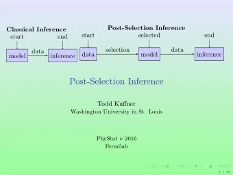
Exact Statistical Inference after Model Selection. Jason D Lee Dept of Statistics and Institute of Computational and Mathematical Engineering, Stanford University Joint work with Jonathan Taylor, Dennis Sun, and Yuekai Sun. February 2014 Jason D Lee Exact Statistical Inference after Model Selection.

Motivation: Linear regression in high dimensions Select relevant variables ˆ S via a variable selection procedure 1 ( k most correlated, lasso, OMP ...). Fit a linear regression model using only the variables in ˆ S . 2 Return the selected set of coefficients ˆ S and the coefficients 3 ˆ β ˆ S . Construct confidence intervals 95% confidence intervals 4 (ˆ β j − 1 . 96 σ j , ˆ β j + 1 . 96 σ j ) . Test the hypothesis H 0 : β j = 0 by rejecting when 5 � � � β j � ≥ 1 . 96 . � � σ j Are these confidence intervals and hypothesis tests correct? Jason D Lee Exact Statistical Inference after Model Selection.

Check by Simulation Generate design matrix X ∈ R n × p from a standard normal with n = 20 and p = 200 . Let y = Xβ 0 + ǫ . ǫ ∼ N (0 , 1) . β 0 is 2 sparse with β 0 1 , β 0 2 = SNR . Use marginal screening to select k = 2 variables, and then fit linear regression over the selected variables. Construct 90% confidence intervals for β and check the coverage proportion. Jason D Lee Exact Statistical Inference after Model Selection.

Simulation 1 Coverage Proportion 0.9 0.8 Adjusted 0.7 Z test 0.6 0.5 0.4 −1 0 1 log 10 SNR Figure: Plot of the coverage proportion across a range of SNR. The coverage proportion of the z intervals is far below the nominal level of 1 − α = . 9 , even at SNR =5. The adjusted intervals (our method) always have coverage proportion . 9 . Jason D Lee Exact Statistical Inference after Model Selection.

Setup Model Assume that y i = µ ( x i ) + ǫ i ǫ i ∼ N (0 , σ 2 ) .   µ ( x 1 ) . x i ∈ R p , y ∈ R n , and µ = .  .   .  µ ( x n ) x T   1 . .  ∈ R n × p . Design matrix X =   .  x T n Jason D Lee Exact Statistical Inference after Model Selection.

Review of Linear Regression The best linear predictor ( f ( x ) = β T x ) is β ⋆ = X † µ . Linear regression estimates this using ˆ β = X † y. Theorem The least squares estimator is distributed β ∼ N ( X † µ, σ 2 ( X T X ) − 1 ) ˆ and β j − zσ ( X T X ) − 1 / 2 β j + zσ ( X T X ) − 1 / 2 � � �� ˆ , ˆ β ⋆ Pr j ∈ = 1 − α. jj jj Jason D Lee Exact Statistical Inference after Model Selection.

Explaining the simulation The confidence intervals rely on the result that ˆ β is Gaussian. 1 The variable selection procedure (marginal screening) chose 2 variables in a way that depend on y . In particular, | X T S y | > | X T S y | . ˆ − ˆ For any fixed set S , X T S y is Gaussian, but X T S y is not 3 ˆ Gaussian! Example Let y ∼ N (0 , I ) , and X = I . Let i ⋆ = arg max y i , then y i ⋆ is not Gaussian. Jason D Lee Exact Statistical Inference after Model Selection.

Condition on selection framework This talk is about a framework for post-selection inference, i.e. the selection procedure is adaptive to the data. The main idea is condition on selection Represent the selection event as a set of affine constraints on 1 y . Derive the conditional distribution and pivotal quantity for 2 linear contrasts η T y . Invert the pivotal quantity to obtain confidence intervals for 3 η T µ . Jason D Lee Exact Statistical Inference after Model Selection.

Motivation 1 Related Work 2 Selection Events 3 Truncated Gaussian Pivotal Quantity 4 Testing and Confidence Intervals 5 Experiments 6 End 7 Jason D Lee Exact Statistical Inference after Model Selection.

Related Work POSI (Berk et al. 2013) widen intervals to simultaneously cover all coefficients of all possible submodels. The method is extremely conservative and is only computationally feasible for p ≤ 30 . Asymptotic normality by “inverting” KKT conditions (Zhang 2012, Buhlmann 2012, Van de Geer 2013, Javanmard 2013). Asymptotic result that requires consistency of the lasso. Significance testing for Lasso (Lockhart et al. 2013) tests for whether all signal variables are found. Our framework allows us to test the same thing with no assumptions on X and is completely non-asymptotic and exact. Jason D Lee Exact Statistical Inference after Model Selection.

Preview of our results The results are exact (non-asymptotic). Only assume X is in general position, and no assumptions on n and p (e.g. n > s log p ). We assume that ǫ is Gaussian and σ 2 is known. The constructed confidence intervals satisfy � � β ⋆ S ∈ [ L j α , U j α ] = 1 − α, Pr j ∈ ˆ S = X † where β ⋆ S µ . j ∈ ˆ ˆ Test for whether the lasso/marginal screening have found all relevant variables. Framework is applicable to many model selection procedures including marginal screening, lasso, OMP, and non-negative least squares. Jason D Lee Exact Statistical Inference after Model Selection.

Marginal screening Algorithm 1 Marginal screening algorithm 1: Input: Design matrix X , response y , and model size k . 2: Compute | X T y | . S be the index of the k largest entries of | X T y | . 3: Let ˆ 4: Compute ˆ S = ( X T S ) − 1 X T β ˆ S X ˆ S y ˆ ˆ Jason D Lee Exact Statistical Inference after Model Selection.

Marginal screening selection event The marginal screening selection event is a subset of R n : � S c � j y , for each i ∈ ˆ S and j ∈ ˆ s i x T i y > ± x T y : ˆ � � y : A ( ˆ s ) y ≤ b ( ˆ = S, ˆ S, ˆ s ) The marginal screening selection event corresponds to selecting a set of variables ˆ S , and those variables having signs � � X T ˆ s = sign S y . ˆ Jason D Lee Exact Statistical Inference after Model Selection.

Lasso selection event Lasso 1 2 � y − Xβ � 2 + λ � β � 1 ˆ β = arg min β KKT conditions provide us with the selection event. A set of variables ˆ S is selected with sign (ˆ β ˆ S ) = ˆ s if � � � � y : sign( U ( ˆ � W ( ˆ = { y : A ( ˆ s ) y ≤ b ( ˆ S, ˆ s )) = z E , S, ˆ s ) ∞ < 1 S, ˆ S, ˆ s ) } � � � where U ( S, s ) := ( X T S X S ) − 1 ( X T S y − λz S ) S ) † z S + 1 W ( S, s ) := X T − S ( X T λX T − S ( I − P S ) y. Jason D Lee Exact Statistical Inference after Model Selection.

Partition via the selection event Partition decomposition We can decompose y in terms of partition, where y is a different constrained Gaussian for each element of the partition. � y ✶ ( A ( S, s ) y ≤ b ( S, s )) y = S,s Theorem The distribution of y conditional on the selection event is a constrained Gaussian, s ) = ( S, s ) } d y |{ ( ˆ = Gaussian constrained to { x : A ( ˆ S, ˆ S, ˆ s ) x ≤ b } . Jason D Lee Exact Statistical Inference after Model Selection.

Motivation 1 Related Work 2 Selection Events 3 Truncated Gaussian Pivotal Quantity 4 Testing and Confidence Intervals 5 Experiments 6 End 7 Jason D Lee Exact Statistical Inference after Model Selection.

Constrained Gaussian The distribution of y ∼ N ( µ, σ 2 I ) conditional on 1 { y : Ay ≤ b } has density Pr ( Ay ≤ b ) φ ( y ; µ, Σ) ✶ ( Ay ≤ b ) . Although we understand the distribution of y condition on selection is a constrained Gaussian, the normalization constant is computationally intractable. We would like to understand the distribution of η T y , since regression coefficients are linear contrasts, ˆ j X † S = e T β j ∈ ˆ S y . ˆ Instead, we show η T y is a (univariate) truncated normal. Jason D Lee Exact Statistical Inference after Model Selection.

Lemma The conditioning set can be rewritten in terms of η T y as follows: { Ay ≤ b } = {V − ( y ) ≤ η T y ≤ V + ( y ) , V 0 ( y ) ≥ 0 } η T Σ η , V 0 = V 0 ( y ) = min j : α j =0 b j − ( Ay ) j , where α = A Σ η b j − ( Ay ) j + α j η T y V − = V − ( y ) = max α j j : α j < 0 b j − ( Ay ) j + α j η T y V + = V + ( y ) = min . α j j : α j > 0 Moreover, ( V + , V − , V 0 ) are independent of η T y . Jason D Lee Exact Statistical Inference after Model Selection.

Geometric Intuition Figure: A picture demonstrating that the set { Ay ≤ b } can be characterized by {V − ≤ η T y ≤ V + } . Assuming Σ = I and || η || 2 = 1 , V − and V + are functions of P η ⊥ y only, which is independent of η T y . Jason D Lee Exact Statistical Inference after Model Selection.

Truncated Normal Corollary The distribution of η T y conditioned on { Ay ≤ b, V + ( y ) = v + , V − ( y ) = v − } is a (univariate) Gaussian truncated to fall between V − and V + , i.e. η T y | { Ay ≤ b, V + ( y ) = v + , V − ( y ) = v − } ∼ TN ( η T µ, η T Σ η, v − , v + ) TN ( µ, σ, a, b ) is the normal distribution truncated to lie between a and b . Jason D Lee Exact Statistical Inference after Model Selection.

Pivotal quantity Theorem Let Φ( x ) denote the CDF of a N (0 , 1) random variable, and let F ( x ; µ, σ 2 , a, b ) denote the CDF of TN ( µ, σ, a, b ) F ( x ; µ, σ 2 , a, b ) = Φ(( x − µ ) /σ ) − Φ(( a − µ ) /σ ) Φ(( b − µ ) /σ ) − Φ(( a − µ ) /σ ) . Then F ( η T y ; η T µ, η T Σ η, V − ( y ) , V + ( y )) is a pivotal quantity F ( η T y ; η T µ, η T Σ η, V − ( y ) , V + ( y )) ∼ Unif (0 , 1) Jason D Lee Exact Statistical Inference after Model Selection.