Evaluation of variance for TCP throughput Olga I. Bogoiavlenskaia - PowerPoint PPT Presentation

Evaluation of variance for TCP throughput Olga I. Bogoiavlenskaia PetrSU, Department of Computer Science olbgvl@cs.karelia.ru

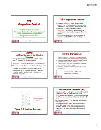
TCP Congestion Control • In distributed packet switching network a sender is not aware about the workload experienced by key elements of the networking environment (links and routers) • Distrubuted flow control is one of the basic networking problems • Congestion collapse 1

TCP Congestion Control • End-to-end transport layer decides which data and when are to be injected in the network and provides delivery control as well • TCP vs UDP • Diversification of the networking applications and the bearers of the signal provide more sophisticated requirements to the flow control algorithms • Reno and NewReno performance defines model behavior for TCP- friendliness (BIC, CUBIC, HTCP, etc) 2

Distributed Flow Control • Data delivery control is done by sliding window and explicit acknowledgme • Sliding window is amount of data which sender is allowed to inject in the network without acknowledgment • Flow control means control on sliding window size. TCP uses set of algorithms to control its window size W Additive Increase Multiplicative Decrease Algorithm (AIMD) delivery W → W + 1 − − − − − ↓ loss W/ 2 3

w(t) w i+1 w i α ’triple−duplicate’ periods w τ τ t td i−1 td td i i+1 i i+1 TCP NewReno ’Saw’ 4

’Root Square’ Lows Let us denote • p TCP segment loss probability • RTT Round Trip Time • RTO Round Trip Timeout • MSS Minimal Segment Size S. Floyd for p ≤ 0 . 025 � 3 T = MSS (1) RTT 2 p D. Towsley group for p > 0 . 025 MSS T = (2) � � 2 p 3 p 8 ) p (1 + 32 p 2 ) RTT 3 + RTOmin (1 , 3 5

Variance evaluation • Throughput variance is nowadays important for many networking applications • Variance is V ar [ X ] = E [ X 2 ] − ( E [ X ] 2 ) • Root square lows are derived thorough Goelders’s inequality i.e. � E [ X 2 ] E [ X ] ≤ 6

Variance evaluation • X 2 n +1 = αX 2 n + 2 bS n , where 0 < α < 1 , b - is growth ratio and S n is amount of data sent without loss • Expanding, one gets n X 2 α 2 i S k + n − i � k + n = 2 b i =0 or � n α 2 i S k + n − i � • X k + n = 2 b i =0 7

Variance evaluation �   n n √ � �� � � � � α 2 i S k + n − i  ≤ α 2 i S k + n − i E [ X k + n ] = E � 2 b 2 b E  i =0 i =0 Transforming to stationary state one gets n √ �� � � α 2 i S i E [ X ] = lim n →∞ E [ X n ] ≤ lim 2 b E = i =0 √ 2 b � 1 − αE [ S n ] For b = 1 and α = 1 2 one gets √ � E [ X ] ≤ 2 2 E [ S n ] 8

Variance evaluation Now we have two estimations of sliding window size expectation � 8 3 E [ S 2 • E [ X ] ≤ A = n ] √ 2 E [ √ S n ] • E [ X ] ≤ B = 2 If B < A then it could be used for estimation variance V ar [ X ] ≤ A 2 − B 2 . This holds if � E [ S n ] � E [ S n ] < . 3 9

Variance evaluation. Examples Lets p.d.f. of S n is F ( x ) = 1 − e λx then E [ S n ] = 1 λ and √ π � 1 � E [ S n ] = λ. 2 Condition does not hold. 10

Variance evaluation Lets p.d.f of S n is Pierson root square distribution then its moments can be calculated through Γ -function and 2 Γ( n +1 2 ) 1 E [ S n ] = 2 Γ( n 2 ) and 4 Γ( 2 n +1 4 ) 1 � E [ S n ] = 2 2 ) . Γ( n The result depends on parameter n. Condition holds for e.g. n = 10 . 11