Equation models versus agent models: an example about pre-crash - PowerPoint PPT Presentation

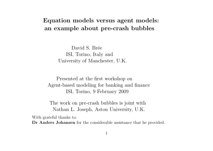
Equation models versus agent models: an example about pre-crash bubbles David S. Br´ ee ISI, Torino, Italy and University of Manchester, U.K. Presented at the first workshop on Agent-based modeling for banking and finance ISI, Torino, 9 February 2009 The work on pre-crash bubbles is joint with Nathan L. Joseph, Aston University, U.K. With grateful thanks to: Dr Anders Johansen for the considerable assistance that he provided. 1

2

In 2005: Lynn, a hard working free-lance translator, inherits a small amount of capital. So that when she has to stop working she will have the rent as a pension, she decides to invest the capital by buying houses-to-let in the attractive nearby town of Kings Lynn, Norfolk, U.K. Then and now ...? 3

4

5

6

7

Understanding versus prediction • Prediction IS understanding: Milton Friedman [video clip] • Understanding without prediction: the literature on the current financial crisis. But see: e.g. Charles Morris, 8

9

• Prediction with understanding: � � p + n 2 a e.g. van der Waals gas laws ( V − nb ) = nRT V 2 where: p is the pressure of the fluid V is the total volume of the container containing the fluid T is the absolute temperature a is a measure of the attraction between the particles a = N 2 A a ′ a ′ is a measure for the attraction between the particles b is the volume excluded by a mole of particles b = N A b ′ b ′ is the average volume excluded from v by a particle n is the number of moles R is the gas constant, R = N A k N A is Avogadro’s constant k is Boltzmann’s constant 10

11

raw HS index with log periodic model fitted on 15 � May � 1989 3500 Data Fitted Predict 3000 Index 2500 3575.313 � 52.509((1989.45 � t)*365) 0.52 [1 � 0.195 cos(4.95 ln((1989.45 � t)*365) � 1.7)] 2000 � today 1987.8 1988 1988.2 1988.4 1988.6 1988.8 1989 1989.2 1989.4 1989.6 Date Figure 1: LPPL fit to the bubble preceding the 1989 crash on Hang Seng

1 The Log Periodic Power Law: y t = A + B ( t c − t ) β � � 1 + C cos( ω log( t c − t ) + φ ) (1) where: y t > 0 is the price (index), or the log of the price; A > 0 the value of y t c at the critical time; B < 0 the increase in y t over the time unit before the crash, if C were to be close to zero; | C | < 1 is the proportional magnitude of the fluctuations around the exponential growth; t c > 0 is the critical time; t < t c is any time into the bubble, preceding t c ; β = 0 . 33 ± 0 . 18 is the exponent of the power law growth; ω = 6 . 36 ± 1 . 56 is the frequency of the fluctuations during the bubble; 0 ≤ φ ≤ 2 π is a shift parameter. 13

Overview: • What is the underlying mechanism? • Is the LPPL with fitted parameters a precursor of crashes? • Are these LPPL parameters sufficient to distinguish between fits that precede a crash from those that do not? [For another occasion] 14

2 The underlying mechanism The martingale condition put forward by Johansen, Ledoit and Sor- nette, 1 is that the expected price rise must be just sufficient to com- pensate for the known risk of a crash: dp = κ.p ( t ) .h ( t ) .dt (2) where: dp is the change in price over the time interval dt ; κ is the proportion by which the price is expected to drop; p ( t ) is the price at time t ; h ( t ) is the hazard rate at time t , i.e. the chance that the crash occurs in the next unit of time, given that it has not occurred already. NB: All the terms on the right hand side of Equation 2 are necessarily positive. 1 Crashes as critical points. International Journal of Theoretical and Applied Finance , 3 , 219–225, 2000. 15

Reordering Equation (2): dp = κ.p ( t ) .h ( t ) .dt gives us: 1 p ( t ) dp = κh ( t ) dt (3) and integrating: � t h ( t ′ ) dt ′ log p ( t ) = κ (4) t 0 Now the behaviour of the hazard rate, h ( t ), needs to be specified. 16

2.1 Traders’ behaviour Johansen et al posit a model in which each trader is in one of two states, either bull (+1) or bear (-1). At the next time step the state, s i , of trader i is given by: � � � s i = sign K s j + σǫ i (5) j ∈ N ( i ) where: K is an imitation factor; N ( i ) is the set of neighbouring traders who influence trader i ; σ is the tendency towards idiosyncratic behaviour amongst all traders; ǫ i is a random draw from a zero mean unit variance from the normal distribution. 17

Further they assume that: - during a bubble the value of K increases, until it reaches a critical value K c ; - this increase is such that K c − K ( t ) depends on t c − t ; - the hazard rate h varies in the same way as K/K c , the suscep- tibility of the collection. With these reasonable, but unfortunately untestable, assumptions, we have the dynamics of the hazard rate: h ( t ) ≈ B ′ ( t c − t ) − α [1 + C ′ cos( ω log( t c − t ) + φ ′ )] (6) 18

Some subsititutions and integration gives us: • Substituting for h in (4) from (6) gives: � t B ′ ( t c − t ′ ) − α { 1+ C ′ cos( ω log( t c − t ′ )+ φ ′ ) } dt ′ (7) log p ( t ) = κ t 0 • Substituting β = 1 − α and ψ ( t ) = ω log( t c − t ) + φ ′ in the integral � � ( t c − t ) − α cos( ω log( t c − t ) + φ ′ ) dt = ( t c − t ) β − 1 cos ψ ( t ) dt = − ( t c − t ) β ω 2 + β 2 { ω sin ψ ( t ) + β cos ψ ( t ) } (8) • Integrating (7) using (8) and substituting: A = log p ( t c ) , B = − κB ′ /β, and C = β 2 C ′ / ( ω 2 + β 2 ), gives us: log p ( t ) ≈ A + B ( t c − t ) β [1 + C cos( ω log( t c − t ) + φ )] (9) which is the LPPL of equation (1) with y t = log( p t ). 19

2.2 Index: raw versus log Johansen et al often fit the LPPL to the raw index rather than the log. • This is justified by replacing the condition (2) by: dp = κ ( p ( t ) − p 1 ) h ( t ) dt (10) where p 1 is some ‘fundamental’ value. • Integrating (10) from the moment when the bubble starts, t 0 , and assuming that p ( t ) − p ( t 0 ) ≪ p ( t 0 ) − p 1 , gives: � t ( p ( t ′ ) − p 1 ) h ( t ′ ) dt ′ p ( t ) = p ( t 0 ) + κ t 0 � t h ( t ′ ) dt ′ . = p ( t 0 ) + κ ( p ( t 0 ) − p 1 ) (11) t 0 20

• This assumption is both untestable and questionable. • There seems to be no underlying justification here for the raw price, rather than its log, to fluctuate as an LPPL. 21

2.3 Tests of the underlying mechanism Chang and Feigenbaum 2 tested the mechanism underlying the LPPL • To do so they first extended the LPPL model by: - adding a random term with zero mean and variance esti- mated from the data. - adding a positive upward drift term, again estimated from the data. • They computed the likelihood, given the extended LPPL model, of the price rises observed for each day. • And not suprisingly found that: the mechanism underlying their adaptation of the LPPL, is not to be preferred above a random walk model. 2 A Bayesian analysis of log-periodic precursors to financial crashes, Quantitative Finance , 6 , 15–36, 2006. 22

But there is another test. Recall that, from Equation 2: dp = κ.p ( t ) .h ( t ) .dt the predicted price must always rise throughout the bubble. In later work Sornette and Zhou used this as a constraint on the parameters But not in the early studies. So was the constraint met in the earlier studies? Recall that it didn’t for the 1989 crash on the Hang Seng: 23

raw HS index with log periodic model fitted on 15 � May � 1989 3500 Data Fitted Predict 3000 Index 2500 3575.313 � 52.509((1989.45 � t)*365) 0.52 [1 � 0.195 cos(4.95 ln((1989.45 � t)*365) � 1.7)] 2000 � today 1987.8 1988 1988.2 1988.4 1988.6 1988.8 1989 1989.2 1989.4 1989.6 Date Figure 2: LPPL fit to the bubble preceding the 1989 crash on Hang Seng

Table 1: Slope of the LPPL fit to the bubbles preceding various crashes, by market and year, from Johansen et al Bubbles ending in crashes where the LPPL fit: Market has a positive slope throughout sometimes has a negative slope Dow Jones 1929, 1962 S&P 1937, 1987 Hang Seng ’71, ’73, ’78, ’80, ’87, ’97 1989, 1994 Korean 1994 Indonesian 1994, 1997 Malaysian 1994 Philippine 1994 Thailand 1994 Argentinian 1994 1991, 1992, 1997 Brazilian 1997 Chilean 1991, 1993 Mexican 1994 1997 Peruvian 1993 1997 Venezuelan 1997 Total number: 14 16 25

So half of the LPPLs fitted to 30 crashes by Johansen et al have a negative slope. This implies that the underlying mechanism is incorrect; but not that the LPPL, with suitable parameters, is a poor fit to bubbles. A potential for saving the underlying mechanism is to insist that the slope is never negative, which is guaranteed by: β 2 + ω 2 ≥ 0 � β − | C | This feature has been used in later work to decide whether or not a LPPL fit was a crash precursor. 3 3 D. Sornette and W.-X. Zhou, Predictability of large future changes in major financial indices. International Journal of Forecasting , 22 , 153-168, 2006. 26

But insisting on this constraint here requires that LPPL fits to half of the bubbles preceding crashes were not crash precursors! 27

3 Is the LPPL with fitted parameters a precur- sor of crashes? • What’s a crash? • Troughs and bubble beginnings. • Fitting the LPPL parameters. [skip] • The ‘best’ fits of the LPPL to the 10 Hang Seng bubbles. 28