Entropy Inference Based on An Objective Bayesian Approach for Upper - PDF document

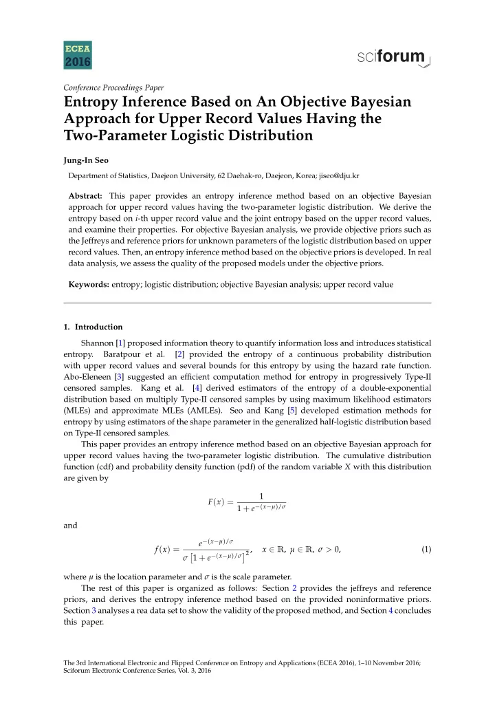
Conference Proceedings Paper Entropy Inference Based on An Objective Bayesian Approach for Upper Record Values Having the Two-Parameter Logistic Distribution Jung-In Seo Department of Statistics, Daejeon University, 62 Daehak-ro, Daejeon, Korea; jiseo@dju.kr Abstract: This paper provides an entropy inference method based on an objective Bayesian approach for upper record values having the two-parameter logistic distribution. We derive the entropy based on i -th upper record value and the joint entropy based on the upper record values, and examine their properties. For objective Bayesian analysis, we provide objective priors such as the Jeffreys and reference priors for unknown parameters of the logistic distribution based on upper record values. Then, an entropy inference method based on the objective priors is developed. In real data analysis, we assess the quality of the proposed models under the objective priors. Keywords: entropy; logistic distribution; objective Bayesian analysis; upper record value 1. Introduction Shannon [1] proposed information theory to quantify information loss and introduces statistical entropy. Baratpour et al. [2] provided the entropy of a continuous probability distribution with upper record values and several bounds for this entropy by using the hazard rate function. Abo-Eleneen [3] suggested an efficient computation method for entropy in progressively Type-II censored samples. Kang et al. [4] derived estimators of the entropy of a double-exponential distribution based on multiply Type-II censored samples by using maximum likelihood estimators (MLEs) and approximate MLEs (AMLEs). Seo and Kang [5] developed estimation methods for entropy by using estimators of the shape parameter in the generalized half-logistic distribution based on Type-II censored samples. This paper provides an entropy inference method based on an objective Bayesian approach for upper record values having the two-parameter logistic distribution. The cumulative distribution function (cdf) and probability density function (pdf) of the random variable X with this distribution are given by 1 F ( x ) = 1 + e − ( x − µ ) / σ and e − ( x − µ ) / σ f ( x ) = 1 + e − ( x − µ ) / σ � 2 , x ∈ ❘ , µ ∈ ❘ , σ > 0, (1) � σ where µ is the location parameter and σ is the scale parameter. The rest of this paper is organized as follows: Section 2 provides the jeffreys and reference priors, and derives the entropy inference method based on the provided noninformative priors. Section 3 analyses a rea data set to show the validity of the proposed method, and Section 4 concludes this paper. The 3rd International Electronic and Flipped Conference on Entropy and Applications (ECEA 2016), 1–10 November 2016; Sciforum Electronic Conference Series, Vol. 3, 2016

The 3rd International Electronic and Flipped Conference on Entropy and Applications (ECEA 2016), 1–10 November 2016; Sciforum Electronic Conference Series, Vol. 3, 2016 2. Objective Bayesian Analysis 2.1. Objective Priors Let X U ( i ) , . . . , X U ( k ) be the upper record values X 1 , . . . , X n from the logistic distribution with pdf (1). Then the corrsponding likelihood function is given by � � f x U ( i ) � k − 1 � ∏ L ( µ , σ ) = f x U ( k ) � � 1 − F x U ( i ) i = 1 � � � � � 1 exp − x U ( k ) − µ / σ � k k 1 ∏ = � . � � � � � � � σ 1 + exp − x U ( k ) − µ / σ 1 + exp − x U ( i ) − µ / σ i = 1 The FIsher information matrix for ( µ , σ ) is given by � ∂ 2 � ∂ 2  � �  E ∂µ 2 log L ( µ , σ ) E ∂µ∂σ log L ( µ , σ )  � ∂ 2 � ∂ 2  I ( µ , σ ) = −  , (2)   � �  E ∂σ∂µ log L ( µ , σ ) E ∂σ 2 log L ( µ , σ ) By the result provided in Asgharzadeh et al. [9], all elements of the Fisher information (2) are proportional to 1/ σ 2 . Therefore, the Jeffreys prior is π J ( µ , σ ) ∝ 1 (3) σ 2 by the definition that it is proportional to the square root of the determinant of the Fisher information. However, the Jeffreys prior has some drawbacks for multi-parameter case such as marginalization paradox, Neyman–Scott problem, and so on. Alternately, Bernardo [10] introduced the reference prior, and Berger and Bernardo [11,12] provided a general algorithm for deriving the reference prior. By using the algorithm, we can obtain the reference prior ( µ , σ ) as π R ( µ , σ ) ∝ 1 σ , (4) regardless which parameter is of interest. Unfortunately, it is impossible to express in closed forms the marginal distribution for µ and σ under the objective priors (3) and (4). To generate the Markov chain Monte Carlo (MCMC) samples from the marginal distributions, we should conduct a MCMC technique. The full conditional posterior distribution for µ and σ under a joint prior π ( µ , σ ) are given by k exp ( µ / σ ) 1 ∏ π ( µ | σ , x ) ∝ π ( µ , σ ) (5) � � � � � � � � 1 + exp − x U ( k ) − µ / σ 1 + exp − x U ( i ) − µ / σ i = 1 and � 1 � � � � − x U ( k ) − µ � k exp / σ k 1 ∏ π ( σ | µ , x ) ∝ π ( µ , σ ) � , (6) � � � � � � � σ 1 + exp − x U ( k ) − µ 1 + exp − x U ( i ) − µ / σ / σ i = 1 respectively. Under both objective priors (3) and (4), the full conditional posterior distribution (5) is log-concave. Therefore, we can draw the MCMC samples µ i ( i = 1, . . . , N ) from the conditional 2

The 3rd International Electronic and Flipped Conference on Entropy and Applications (ECEA 2016), 1–10 November 2016; Sciforum Electronic Conference Series, Vol. 3, 2016 posterior distribution (5) by using the method proposed by Devroye [13]. We also need to note the fact that σ ∈ ❘ + , but µ ∈ ❘ and X U ( i ) ∈ ❘ . In this case, it is not easy to find a suitable proposal distribution for drawing the MCMC samples σ i ( i = 1, . . . , N ) from the full conditional posterior distribution (6). Therefore, we employ the random-walk Metropolis algorithm based on a normal proposal distribution truncated at zero. 2.2. Entropy Theorem 1. The entropy based on ith upper record value X U ( i ) is ∞ 1 ∑ H U ( i ) = log Γ ( i ) + log σ + i − ( i − 1 ) ψ ( i ) + j ( j + 1 ) i . (7) j = 1 Remark 1. It is clear that the entropy (7) is an increasing function of σ . Therefore, the larger σ , the less information is provided by the distribution due to increasing entropy. Remark 2. We can obtain the following relationships between two adjacent entropies: � �� ∞ � 1 1 � � ∑ lim H U ( i + 1 ) − H U ( i ) = lim log ( i − 1 ) − ψ ( i − 1 ) + j ( j + 1 ) i − j ( j + 1 ) i − 1 i → ∞ i → ∞ j = 1 � ∞ ��� �� 1 � � 1 ∑ = lim − log 1 + i − 1 + j i − 1 + j i → ∞ j = 0 = 0. Theorem 2. The joint entropy based on X U ( 1 ) , . . . , X U ( k ) is ∞ k 1 ∑ ∑ H U ( 1 ) ,..., U ( k ) = k ( 1 + log σ ) + j ( j + 1 ) i , (8) i = 1 j = 1 which is an increasing function of σ as Remaek 1. Proof. The joint entropy based on upper record values X U ( 1 ) , . . . , X U ( k ) is defined by Park [14] as � ∞ � x U ( 2 ) H U ( 1 ) ,..., U ( k ) = − − ∞ · · · f X U ( 1 ) ,..., X U ( k ) ( x U ( 1 ) ,..., x U ( k ) ) − ∞ × log f X U ( 1 ) ,..., X U ( k ) ( x U ( 1 ) ,..., x U ( k ) ) dx U ( 1 ) , . . . , dx U ( k ) , where f X U ( 1 ) ,..., X U ( k ) ( x U ( 1 ) ,..., x U ( k ) ) is the joint density function of x U ( 1 ) , . . . , x U ( k ) . In addition, it is simplified to a single-integral by Rad et al. [15] as � ∞ k H U ( 1 ) ,..., U ( k ) = k ( 1 − k ) 1 Γ ( i ) [ − log ( 1 − F ( x ))] i − 1 f ( x ) log f ( x ) dx ∑ − (9) 2 − ∞ i = 1 Then the integral term in (9) is given by � ∞ � ∞ 1 Γ ( i ) [ − log ( 1 − F ( x ))] i − 1 f ( x ) log f ( x ) dx = − log σ − 2 y i e − y dy − ∞ 0 � ∞ y i − 1 e − y log ( e y − 1 ) dy + 0 3