Entity Resolution with Weighted Constraints Zeyu Shen and Qing Wang - PowerPoint PPT Presentation
Entity Resolution with Weighted Constraints Zeyu Shen and Qing Wang Research School of Computer Science Australian National University Australia qing.wang@anu.edu.au 2 Entity Resolution Entity resolution (ER) is to determine whether or
Entity Resolution with Weighted Constraints Zeyu Shen and Qing Wang Research School of Computer Science Australian National University Australia qing.wang@anu.edu.au 2
Entity Resolution • Entity resolution (ER) is to determine whether or not different entity represen- tations (e.g., records) correspond to the same real-world entity. 3
Entity Resolution • Entity resolution (ER) is to determine whether or not different entity represen- tations (e.g., records) correspond to the same real-world entity. • Consider the following relation Authors : ID Name Department University i 1 Peter Lee Department of Philosophy University of Otago i 2 Peter Norrish Science Centre University of Otago i 3 Peter Lee School of Philosophy Massey University i 4 Peter Lee Science Centre University of Otago • Questions: – Are Peter Lee ( i 1 ) and Peter Lee ( i 3 ) the same person? – Are Peter Norrish ( i 2 ) and Peter Lee ( i 4 ) not the same person? – . . . 4
State of The Art • State-of-the-art approaches to entity resolution favor similarity-based methods. 5
State of The Art • State-of-the-art approaches to entity resolution favor similarity-based methods. • Numerous techniques under a variety of perspectives: a. threshold-based b.cost-based c. rule-based d.supervised e. active learning f. clustering-based g. . . . 6
State of The Art • State-of-the-art approaches to entity resolution favor similarity-based methods. • Numerous techniques under a variety of perspectives: a. threshold-based b.cost-based c. rule-based d.supervised e. active learning f. clustering-based g. . . . • The central idea is “The more similar two entity representations are, the more likely they refer to the same real-world entity.” 7
Goal of this Paper • To study entity resolution in the presence of constraints, i.e., ER constraints. 8
Goal of this Paper • To study entity resolution in the presence of constraints, i.e., ER constraints. • ER constraints ubiquitously exist in real-life applications. (1) “ ICDM” refers to “IEEE International Conference on Data Mining” and vice versa (Instance level). (2) Two paper records refer to different papers if they do not have the same page numbers (Schema level). 9
Goal of this Paper • To study entity resolution in the presence of constraints, i.e., ER constraints. • ER constraints ubiquitously exist in real-life applications. (1) “ ICDM” refers to “IEEE International Conference on Data Mining” and vice versa (Instance level). (2) Two paper records refer to different papers if they do not have the same page numbers (Schema level). • They allow us to leverage rich domain semantics for improved ER quality. • Such constraints can be obtained from a variety of sources: a. background knowledge, b. external data sources, c. domain experts, d. . . . 10
Research Questions • We study two questions on ER constraints: (1) How to effectively specify ER constraints? (2) How to efficiently use ER constraints? 11
Research Questions • We study two questions on ER constraints: (1) How to effectively specify ER constraints? (2) How to efficiently use ER constraints? • Our task is incorporate semantic capabilities (in form of ER constraints) into existing ER algorithms to improve the quality, while still being computationally efficient. 12
Research Questions • We study two questions on ER constraints: (1) How to effectively specify ER constraints? (2) How to efficiently use ER constraints? • Our task is incorporate semantic capabilities (in form of ER constraints) into existing ER algorithms to improve the quality, while still being computationally efficient. • A key ingredient is to associate each constraint with a weight that indicates the confidence on the robustness of semantic knowledge it represents. Not all constraints are equally important. 13
An Example A database schema paper := { pid, authors, title, journal, volume, pages, tech, booktitle, year } author := { aid, pid, name, order } venue := { vid, pid, name } Views title := π pid,title paper hasvenue := π pid,vid venue pages := π pid,pages paper vname := π vid,name venue publish := π aid,pid,order author aname := π aid,name author Constraints Weights paper ∗ ( x, y ) ← title ( x, t ) , title ( y, t ′ ) , t ≈ 0 . 8 t ′ r 1 : 0.88 paper ∗ ( x, y ) ← title ( x, t ) , title ( y, t ′ ) , t ≈ 0 . 6 t ′ , sameauthors ( x, y ) r 2 : 0.85 paper ∗ ( x, y ) ← title ( x, t ) , title ( y, t ′ ) , t ≈ 0 . 7 t ′ , hasvenue ( x, z ) , r 3 : hasvenue ( y, z ′ ) , venue ∗ ( z, z ′ ) 0.95 ¬ paper ∗ ( x, y ) ← pages ( x, z ) , pages ( y, z ′ ) , ¬ z ≈ 0 . 5 z ′ r 4 : 1.00 venue ∗ ( x, y ) ← hasvenue ( z, x ) , hasvenue ( z ′ , y ) , paper ∗ ( z, z ′ ) r 5 : 0.75 venue ∗ ( x, y ) ← vname ( x, n 1 ) , vname ( y, n 2 ) , n 1 ≈ 0 . 8 n 2 r 6 : 0.70 r 7 : ¬ author ∗ ( x, y ) ← publish ( x, z, o ) , publish ( y, z ′ , o ′ ) , paper ∗ ( z, z ′ ) , o ̸ = o ′ 0.90 author ∗ ( x, y ) ← coauthorML ( x, y ) , ¬ cannot ( x, y ) r 8 : 0.80 14
Learning Constraints • Two-step process: • Specify ground rules to capture the semantic relationships, which may have different interpretations for similarity atoms in different applications. paper ∗ ( x, y ) ← title ( x, t ) , title ( y, t ′ ) , t ≈ λ t ′ g 1 : 15
Learning Constraints • Two-step process: • Specify ground rules to capture the semantic relationship, which may have different interpretations for similarity atoms in different applications. paper ∗ ( x, y ) ← title ( x, t ) , title ( y, t ′ ) , t ≈ λ t ′ g 1 : • Refine ground rules into the “best” ones for specific applications by learning. (1). paper ∗ ( x, y ) ← title ( x, t ) , title ( y, t ′ ) , t ≈ 0 . 8 t ′ ; (2). paper ∗ ( x, y ) ← title ( x, t ) , title ( y, t ′ ) , t ≈ 0 . 7 t ′ ; (3). . . . 16
Learning Constraints • Positive and negative rules have different metrics α and β : Positive rules Negative rules tp tn α tp + fp tn + fn tp tn β tp + fn fp + tn 17
Learning Constraints • Positive and negative rules have different metrics α and β : Positive rules Negative rules tp tn α tp + fp tn + fn tp tn β tp + fn fp + tn • Objective functions must be deterministic and monotonic . – Soft rules max λ ξ ( α, β ) subject to α ≥ α min and β ≥ β min . – Hard rules max λ ξ ( α, β ) subject to w ≥ 1 − ε . 18
Using Constraints • ER matching: To obtain ER graphs G = ( V, E, ℓ ), each having a set of matches ( u, v ) = or non-matches ( u, v ) ̸ = , together with a weight ℓ ( u, v ) for each match and non-match. • ER clustering: Given an ER graph G = ( V, E, ℓ ), to find a valid clustering over G such that vertices are grouped into one cluster iff their records represent the same real-world entity. ER Constraints ER Matching ER Cluste ring ER Propagation 19
Using Constraints - ER Matching • Soft rules with one hard rule: ℓ ( u, v ) = ⊤ or ℓ ( u, v ) = ⊥ rule match/non-match weight ℓ ( u, v ) = ⊥ ( u, v ) = r 1 ω ( r 1 ) = 0 . 88 ��� ( u, v ) = (a hard edge r 3 ω ( r 3 ) = 0 . 95 ( u, v ) ̸ = between u and v ) r 4 ω ( r 4 ) = 1 20
Using Constraints - ER Matching • Soft rules with one hard rule: ℓ ( u, v ) = ⊤ or ℓ ( u, v ) = ⊥ rule match/non-match weight ℓ ( u, v ) = ⊥ ( u, v ) = r 1 ω ( r 1 ) = 0 . 88 ��� ( u, v ) = (a hard edge r 3 ω ( r 3 ) = 0 . 95 ( u, v ) ̸ = between u and v ) r 4 ω ( r 4 ) = 1 • Only soft rules: ℓ ( u, v ) ∈ [0 , 1] rule match/non-match weight ℓ ( u, v ) = 0 . 215 ( u, v ) = r 1 ω ( r 1 ) = 0 . 88 ��� ( u, v ) = (a soft edge between r 3 ω ( r 3 ) = 0 . 95 ( u, v ) ̸ = u and v ) r 9 ω ( r 4 ) = 0 . 70 21
Using Constraints – ER Clustering • A natural view is to use correlation clustering techniques. • Clustering objectives are often defined as minimizing disagreements or maxi- mizing agreements. • However, it is known that correlation clustering is a NP-hard problem. • Two approaches we will explore: – Pairwise nearest neighbour (PNN) – Relative constrained neighbour (RCN) 22
Pairwise Nearest Neighbour • Iteratively, a pair of two clusters that have the strongest positive evidence is merged, until the total weight of edges within clusters is maximized. 1 1,3,4 1,3 0.6 0.9 3 1.3 0.8 0.7 0.8 0.8 4 2 4 2 2 • Negative soft edges are “hardened” into negative hard edges under certain con- ditions. 23
Relative Constrained Neighbour • Iteratively, a cluster that contains hard edges ⊥ is split into two clusters based on the weights of relative constrained neighbours. 1 1 1,3 0.6 0.9 0.9 3 3 0.8 0.7 0.8 0.8 4 4 2 2 2,4 • Negative soft edges are “hardened” into negative hard edges under certain con- ditions. 24
Experimental Study • We focused on three aspects: - ER models: How effectively can constraints and their weights be learned from domain knowledge for an ER model? - ER clustering: How useful can weighted constraints be for improving the ER quality? - ER scalability: How scalable can our method be over large data sets? 25
Recommend
More recommend
Explore More Topics
Stay informed with curated content and fresh updates.
