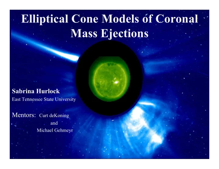
Elliptical Cone Models of Coronal Mass Ejections Sabrina Hurlock - PowerPoint PPT Presentation

Elliptical Cone Models of Coronal Mass Ejections Sabrina Hurlock East Tennessee State University Mentors: Curt deKoning and Michael Gehmeyr

My Mission To boldly go…  To make an IDL version of the Elliptical Cone Model.  To take data from the SOHO/LASCO database, fit an ellipse to the observed CME data, and input ellipse parameters into the IDL cone model program.  Compare model results to the observed data.

Why Study CMEs? To understand the effects on:  Satellites (GPS, cell phones, etc)  Power  Astronauts

SOHO/LASCO Database  CME data taken from 1996 to the present  Tells which coronagraph was used: C2 and/or C3  Tells whether or not the event was strong or weak  Tells us what type of CME occurred, i.e., halo and partial halo

Why Use Cone Models? Tell us about several characteristics of the CME such as:  The shape of the CME, i.e., whether it is narrow at the vertex and has a long radial axis or if it is wide at the vertex and has a short radial axis.  What direction the CME is moving.  The 3D speed of the CME.

Zhao’s Circular Cone Model  Deals with CMEs in the shape of a circular cone.  Equations that describe the cone X c =s*cos( ω ) =r Y c =s*sin( ω )*cos( δ ) Z c =s*sin( ω )*sin( δ )  Delta is parameter that ranges from 0 to 360 degrees.

Zhao’s Model cont’d  The plane of the sky is given by Y h Z h .  The cone’s base is projected on the plane of the sky by: Y h =X c *sin( λ )*sin( ϕ )+Y c *cos( ϕ )-Z c *sin( λ )*sin( ϕ ) Z h =X c *sin( λ )+Z c *cos( λ )  So, what’s the problem? It does not fit the data!  However, Zhao’s model served as the basis for the Elliptical Cone Model.

Elliptical Cone Model  Deals with CMEs in the shape of an elliptical cone.  Same basic principle as Zhao’s model, only more complicated.  Now have to deal with two half-angular widths ; one for the semi minor axis ( ω a ) and one for the semi major axis ( ω b ).  Because of the two half-angular widths, there are now also two slant heights that are related by: s a *cos( ω a ) =s b *cos( ω b ) =r

Elliptical Cone Model  We also have to worry about the tilt of the semi major axis, given by χ , with respect to the Y c axis. Note that the X c axis is pointing out of the screen.  The equations that define the cone are: X c =s a *cos( ω a ) Y c ( δ )=s b *sin( ω b )*cos( δ )*cos( χ )+s a *sin( ω a )*sin( δ )*sin( χ ) Z c ( δ )=s a *sin( ω a )*sin( δ )*cos( χ )-s b *sin( ω b )*cos( δ )*sin( χ )

Elliptical Cone Model Finding the Equation of the Ellipse  Use five points that are located around the leading edge of the CME and plug into the IDL program (this is much more complicated, so we do not use it!).

Elliptical Cone Model Finding the Equation of the Ellipse  Goal One: Find the coordinates of the source region.  We need this to eventually narrow down the number of cone models.  Used the IDL “Fit_Ellipse” program to find the coordinates.

Elliptical Cone Model Finding the Equation of the Ellipse  Trace around the leading edge of the CME using an IDL program called “Fit_Ellipse,” that will give you the equation.

The Elliptical Cone Model Finding the Equation of the Ellipse These calculations give us: • Tilt of semi-major axis which is given by Ψ . • The lengths of the semi minor (a) and semi major (b) axes. • The coordinates for the center of the ellipse, [h,k]. • From these calculations we can find the parametric equation of the ellipse: y p ( δ )=h-a*cos( Ψ )*cos( δ )+b*sin( Ψ )*sin( δ ) z p ( δ )=k-a*sin( Ψ )*cos( δ )-b*cos( Ψ )*sin( δ )

Elliptical Cone Model Cone Parameters  Next, we match equations for the projection of the cone’s base on the sky Y h =X c *sin( λ )*sin( ϕ )+Y c *cos( ϕ )-Z c *sin( λ )*sin( ϕ ) Z h =X c *sin( λ )+Z c *cos( λ ) with the ellipse’s parametric equation that the model gave us y p ( δ )=h-a*cos( Ψ )*cos( δ )+b*sin( Ψ )*sin( δ ) z p ( δ )=k-a*sin( Ψ )*cos( δ )-b*cos( Ψ )*sin( δ to get a system of equations with six unknowns: h=s a *cos( ω a )*cos( λ )*sin( ϕ ) -a*cos( Ψ )=s b *sin( ω b )*[cos( ϕ )*cos( χ )+sin( λ )*sin( ϕ )*sin( χ )] b*sin( Ψ )=s a *sin( ω a )*[cos( ϕ )*sin( χ )-sin( λ )*sin( ϕ )*cos( χ )] k=s b *cos( ω b )*cos( λ ) a*sin( Ψ )=s b *sin( ω b )* cos( λ )*sin( χ ) -b*cos( Ψ )=s a *sin( ω a )* cos( λ )*cos( χ )

Elliptical Cone Model Cone Parameters  The six unknowns from the previous equations are ϕ , λ , χ , r, ω a , and ω b (where ϕ and λ are the heliographic longitude and latitude, χ is the tilt of the semi major axis, r is the radial distance from the sun to the edge of the CME through the central axis, and ω a and ω b are the half-angular widths of the semi minor/major axes)  To find these numerical solutions, we must introduce yet another variable called δ 2. This is a phase angle that ranges from 0 to 360 degrees.  By replacing the left side of the six previous equations with x i , X 0 =h X 1 = - a*cos( Ψ )*cos( δ 2)+b*sin( Ψ )*sin( δ 2) X 2 = a*cos( Ψ )*sin( δ 2)+b*sin( Ψ )*cos( δ 2) X 3 =k X 4 = -a*sin( Ψ )*cos( δ 2)-b*cos( Ψ )*sin( δ 2) X 5 = a*sin( Ψ )*sin( δ 2)-b*cos( Ψ )*cos( δ 2)

Elliptical Cone Model Cone Parameters  We can incorporate the x i values into the following equations to solve for numerical the six unknown parameters. Φ =arcsin λ =arctan χ =arctan ω a =arctan

Elliptical Cone Model Cone Parameters ω b =arctan s a = s b =  After calculating these values, we can make plots of the ellipses.

Testing the Model  Using the “Fit_Ellipse” program, we found the ellipse’s parametric equation and then fed the equation into another IDL program called “Ellipse_Parameters”, written by Curt deKoning, to get the values of the semi major and semi minor axes, and the tilt of the semi major axis.  We then input those parameters into the second part of the IDL program, coincidentally called “Elliptical_Cone_Model_Part2,” to find the characteristics of the cone.  We compared the values we acquired for λ and ϕ (heliographic latitude and longitude) and r (radial distance of the cone) to the actual values, thus eliminating MANY of the cones.

Data http://cdaw.gsfc.nasa.gov/CME_list/daily_m ovies/2006/12/13/c2eit.html

Data

The Results  Plotting the parametric equation for each value of δ 2 gave us the exact same ellipse!  The following movie is a compilation of all 360 δ 2 parameters when plugged into the parametric equation of the ellipse.  PLAY MOVIE!

The Results  The next step is to manually go through all of the values for ϕ and λ (the heliographic latitude and longitude) to see if there are any values that match up with actual coordinates of the CME’s source region.  This effectively eliminates many of the cone models.  After this, we need to look at the radial distance (the height of the CME) to see if there are any extreme values, such as a CME that extends beyond the distance from the Sun to the Earth.

The Results

The Results

The Results

The Results We used the relationship V= Δ x to find the velocity of the CME as it moved outward from Δ t the sun. Then a miracle occurred? The velocity came out as a negative number! That’s when we realized there was something wrong somewhere in our IDL code.

Future Work  Find the error in the IDL code.  Reduce number of models to get a manageable number of cones.  Run more models!

Acknowledgements  Curt deKoning  Michael Gehmeyer  SWPC: Doug Biesecker and Chris Balch  Marty Snow  LASP