Efficiently Mining Long Patterns from Databases Roberto Bayardo - PowerPoint PPT Presentation
Efficiently Mining Long Patterns from Databases Roberto Bayardo IBM Almaden Research Center 1 of 22 The Problem Current flock of algorithms for mining frequent itemsets in databases: Use (almost exclusively) subset-infrequency pruning -
Efficiently Mining Long Patterns from Databases Roberto Bayardo IBM Almaden Research Center 1 of 22
The Problem Current flock of algorithms for mining frequent itemsets in databases: • Use (almost exclusively) subset-infrequency pruning - An itemset is frequent if and only if all its subsets are frequent - Example: Apriori will check eggs&bread&butter only after eggs&bread, eggs&butter, and bread&butter are known to be frequent • Scale exponentially (in time and space) in length of longest frequent itemset • Complexity becomes problematic on many data-sets outside the domain of market-basket analysis - Several classification benchmarks [Bayardo 97] - Census data [Brin et al., 97] 2 of 22
Talk Overview • Show how to incorporate superset-frequency based pruning into a search for maximal frequent itemsets - If an itemset is known to be frequent, then so are its subsets • Define a technique for lower-bounding the frequency of an itemset using known frequencies of its proper subsets • Incorporate frequency-lower-bounding into the maximal frequent-itemset finding algorithm (producing Max- Miner) as well as Apriori (producing Apriori-LB) • Experimental evaluation • Conclusion & Future Work 3 of 22
Some Quick Definitions We are focusing on the problem of finding maximal frequent itemsets in transactional databases. • A transaction is a database entity composed of a set of items, e.g. the supermarket items purchased by a customer during a shopping visit. • The support of a set of items (or itemset ) is the number of transactions in the database to contain it. • An itemset is frequent if its support exceeds a user- defined threshold (minsup). Otherwise it is infrequent . • An itemset is maximal frequent if no superset of it is frequent. 4 of 22
Pruning with Superset-Frequency Some previous work has investigated the idea in the context of identifying maximal frequent itemsets in data: • Gunopulos et al. [ICDT-97] • Memory resident data limitation • Evaluated primarily an incomplete algorithm • Zaki [KDD-97] • Superset-frequency pruning limited in its application • Does not scale to long frequent itemsets • Lin & Kedem [EDBT-98] • Concurrent proposal • Uses NP-hard candidate generation scheme 5 of 22
My Approach • Explicitly formulate the search for frequent itemsets as a tree search (instead of lattice search) problem. • Use both superset-frequency and subset-infrequency to prune branches and nodes of the tree. • Dynamically reorganize the search tree to (heuristically) maximize pruning effectiveness. 6 of 22
Set-Enumeration Tree Search • Impose an ordering on the set of items. • Root node is the empty set. • Children of a node are formed by appending an item that follows all existing node items in the item ordering. • Each and every itemset enumerated exactly once. {} 1 2 3 4 1,2 1,3 1,4 2,3 2,4 3,4 1,2,4 1,3,4 2,3,4 1,2,3 1,2,3,4 • Key to efficient search: Pruning strategies applied to remove nodes and sub-trees from consideration. 7 of 22
Node Representation • To facilitate pruning and other optimizations, we represent each node g in the SE-tree as a candidate group consisting of: • The itemset represented by the node, called the head and denoted h g ( ) . • The set of viable items that can be appended to the head to form the node’s children, called the tail and denoted ( ) t g . • By “computing the support” of a candidate group g , I mean computing the support of not only ( ) , but also: h g ∪ ∈ • ( ) for all ( ) h g i i t g ∪ • h g ( ) t g ( ) (called the long itemset of a candidate group). 8 of 22
Example { , } { , , } At node where ( ) = 1 2 and ( ) = 3 4 5 g h g t g { , , } { , , } { , , } • Compute the support of 1 2 3 , 1 2 4 , 1 2 5 . • Used for subset-infrequency based pruning. { , , } • For example, if 1 2 4 is infrequent, then 4 is not viable . • Children of a node need only inherit viable tail items. { , , , , } • Compute the support of 1 2 3 4 5 • Used for superset-frequency based pruning. { , , , , } • For example, if 1 2 3 4 5 is frequent, then so are all other children of g . 9 of 22
Algorithm (Max-Miner) initialized to contain one group with an empty head. C • initialized to empty. M • • While non-empty: C • Compute the support of all candidate groups in . C ∈ • For each g C with a long itemset that is frequent, ∪ put ( ) ( ) in . h g t g M ∈ • For every other g C , generate children of g If has no children, then put ( ) in . g h g M • Let C contain the newly generated children. • Remove sets in M with supersets, and return M . 10 of 22
Generating Children To generate children of a candidate group : g ∪ • Remove any tail item from ( ) if ( ) is i t g h g i infrequent. • Impose a new order on the remaining tail items. • For each remaining tail item i Generate a child g ' with: ∪ { } • h g ' ( ) = h g ( ) i { } • t g ' ( ) = j j follows i in t g ( ) 11 of 22
Example ( ) { , } { , , , } = 1 2 , ( ) = 3 4 5 6 : h g t g { , , } { , , } ( ) = 1 2 3 , ( ) = 4 5 6 h g 1 t g 1 • { , , } { , } ( ) = 1 2 4 , ( ) = 5 6 h g 2 t g 2 • { , , } { } ( ) = 1 2 5 , ( ) = 6 h g 3 t g 3 • { , , } { } h g 4 ( ) = 1 2 6 , t g 6 ( ) = • 12 of 22
Item Ordering • Goal: Maximize pruning effectiveness. • Strategy: Order tail items in increasing order of support ( ) ∪ { } relative to the head, sup h g ( ) . i • Forces candidate groups with long tails to have heads with low support. • Forces most-frequent items to appear more frequently in the tails of candidate groups. • This is a critical optimization! 13 of 22
Support Lower-Bounding • Idea is to use the support information provided by an itemset’s proper subsets to lower-bound its support. • If the itemset’s support can be lower-bounded above minsup, then it is known to be frequent without requiring database access. • Support lower-bounding can be used to avoid overhead associated with computing the support of many candidate itemsets. 14 of 22
Support Lower-bounding: Theory , ∪ { } • Definition: drop I s j ( ) = sup I s ( ) – sup I s ( ) j I s I ∪ { } I s j ∪ { } I j , , • Note that drop I s j ( ) is an upper-bound on drop I j ( ) ∪ { } , • Note that sup I ( j ) = sup I ( ) – drop I j ( ) , • Theorem: sup I ( ) – drop I s j ( ) is a lower-bound on the ∪ { } support of I j . 15 of 22
Exploiting Support Lower-Bounds To generate children of a candidate group : g ∪ • Remove any tail item from ( ) if ( ) is i t g h g i infrequent. • Impose a new order on the remaining tail items. • For each remaining tail item in increasing item order i do: Generate a child g ' with: ∪ { } • h g ' ( ) = ( ) h g i { } • t g ' ( ) = j j follows i in t g ( ) ∪ • if Compute-Lower-Bound( h g ' ( ) t g ' ( ) ) >= minsup, ∪ then return h g ' ( ) t g ' ( ) to be put in M 16 of 22
Lower-bounding in Apriori • Modify Apriori so that it only computes the support of candidate itemsets that were not found frequent through lower-bounding. • We call the resulting algorithm Apriori-LB. 17 of 22
Results: Census Data 100000 Max-Miner Apriori-LB Apriori 10000 CPU Time (sec) 1000 100 10 35 30 25 20 15 10 5 Support (%) 18 of 22
Scaling (external slide) 19 of 22
DB Passes 40 census* chess 35 connect-4 splice mushroom 30 retail DB passes 25 20 15 10 5 5 10 15 20 25 30 35 40 Length of longest pattern 20 of 22
Conclusions • Long maximal frequent itemsets can be efficiently mined from large data-sets. • Key idea: Superset-frequency based pruning applied heuristically throughout the search. • Support lower-bounding is effective at substantially reducing the candidate groups considered by Max-Miner. • Support lower-bounding is effective at reducing candidate itemsets checked against the database in Apriori. 21 of 22
Future Work • Integrating additional constraints into the search: • Association rule confidence • Rule “interestingness” measures • Goal: Be able to mine association rules instead of maximal-frequent itemsets from long-pattern data. • Apply ideas to mining other patterns • sequential patterns • frequent episodes 22 of 22
Recommend
More recommend
Explore More Topics
Stay informed with curated content and fresh updates.

