ECE 4524 Artificial Intelligence and Engineering Applications - PowerPoint PPT Presentation

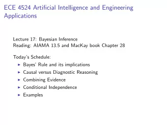
ECE 4524 Artificial Intelligence and Engineering Applications Lecture 16: Uncertainty and Probability Reading: AIAMA 13.1.-13.4 Today’s Schedule: ◮ Probability Refresher ◮ Reasoning and Decisions under Uncertainty ◮ Probabilistic Inference ◮ Independence and Factoring

What about the world is uncertain? ◮ Sometimes events themselves are uncertain ◮ More often, uncertainty is lack of information ◮ Real environments are not fully observable

Motivation: Warmup problem A widely-known problem in probability theory is the Monte Hall problem. There are three doors with a prize behind one and nothing behind the others. If you choose the door with the prize you get it. You are asked to choose a door, then another door without the prize is opened. You are given the opportunity to change your mind and switch doors. You should do so, True or False.

Probability Theory Probability theory begins with { Ω , A , P } ◮ Ω is the sample space ◮ A is a σ -algebra on Ω, the set of all possible events ◮ P : A → [0 , 1] is the probability measure on A Kolmogorov’s axioms lay the foundation 1. P ≥ 0 2. P (Ω) = 1 3. for a countable sequence of disjoint sets in A A 1 , A 2 , · · · P ( A 1 ∪ A 2 ∪ · · · ) = � ∞ i =1 P ( A i )

Warmup #2 In the Monte-Hall Problem what are the events and sample space?

Random Variables A random variable (r.v.), X is a mapping from Ω onto a set T X : Ω → T written as X ( ω ) for ω ∈ Ω where T is a subset of the integers, real numbers, or a mixture. Examples ◮ for a discrete r.v. T is a subset of integers ◮ for a continuous r.v. T is a subset of the real numbers ω is referred to as a sample .

Discrete R.V.s For discrete r.v., X , we work with the distribution (law, or probability mass function, PMF) P X ( x ) = P [ X ( ω ) = x ] for x ∈ T for T a subset of the integers. ◮ 0 ≤ P X ( x ) ≤ 1 ◮ � x ∈ T P X ( x ) = 1

Continuous R.V.s For continuous r.v., X , we work with the distribution function, F X ( x ) F X ( x ) = P [ X ( ω ) < x ] for x ∈ T for T a subset of the real numbers. ◮ 0 ≤ F X ( x ) ≤ 1 ◮ F X ( −∞ ) = 0 and F X ( ∞ ) = 1 and the probability density function (PDF), f X ( x ) � x F X ( x ) = f X ( u ) du −∞ ◮ f X ( x ) ≥ 0 ◮ � ∞ −∞ f X ( u ) du = 1

PMF’s and PDFs are the tools used to specify the knowledge base and make queries. ◮ Agent models have different state variables, X , Y , Z , · · · ◮ The joint density tells us everything we need to know to do probabilistic inference. ◮ Marginalization is used to average over variables we know little about ◮ Conditioning is used when we know one of the variables ◮ Independence allows the joint density to be factored.

Why is probability the right tool for reasoning under uncertainty? Richard Cox postulated three criteria for ”logical probability” 1. The plausibility of a statement is a real number and is dependent on information we have related to the statement (divisibility and comparability). 2. Plausibilities should vary sensibly with the assessment of plausibilities in the model (common sense). 3. If the plausibility of a statement can be derived in many ways, all the results must be equal (consistency). These ideas were taken up (e.g. E.T. Jaynes) and formalized using probability theory to obtain Bayesian Probability Theory or the Bayesian interpretation of probability.

Frequentist versus Bayesian interpretation ◮ The frequentist view is that P is a ratio of the frequency of the specific event relative to the total number of observed events ◮ The Bayesian view is that P is a measure of the degree-of-belief given some evidence Both views are equally correct, both are useful, and they can be used together ◮ Frequentist procedures look like R ( θ ) = E [ L ( δ ( D ) , θ )] ◮ Bayesian procedures look like ρ ( D ) = E [ L ( δ ( D ) , θ )] Bayesian approaches dominate in AI to build the decision process, δ . Frequentist approaches are useful for validating those processes using experiments.

Lets define a probability of an event is a measure of the degree-of-belief in the event given the evidence, or data. P ( E | D ) P ( E | D ) == 0 means the event is impossible, P ( E | D ) == 1 means the event is certain ◮ if the evidence changes so does the belief (except for impossible and certain events) ◮ if two observers have different evidence they will have different beliefs ◮ thus the belief is subjective in that it depends on the evidence, ◮ but two rational observers given the same evidence have the same belief

Some useful nomenclature Let θ be a variable of interest and D be some data (observations) ◮ a model, m , is a way to generate the data parameterized by (indexed by) θ ◮ P [ D | m , θ ] is the likelihood ◮ P [ θ | m ] is the prior ◮ P [ D | m ] is the evidence for the model m (also called the marginal liklihood) ◮ P [ θ | D , m ] is the posterior . Where P above may be a probability, a distribution, or a density.

How does logical reasoning about state variables relate to probabilistic inference? ◮ in logic we ASK(X), where X is a proposition or a definite clause, and get back yes it can be inferred or no it cannot ◮ in logical probability as ASK(X), where X is a r.v. and get back a probability or a density. The process of inference is how to obtain some probabilities, the query, given the knowledge base, the joint probability.

Next Actions ◮ Reading on Bayesian Reasoning, AIAMA 13.5 ◮ Complete warmup before noon on Tu 3/20 Reminder: PS 3 is released. Due 4/5.