Dynamics of Non-densely Defined Stochastic Evolution Equations - PowerPoint PPT Presentation

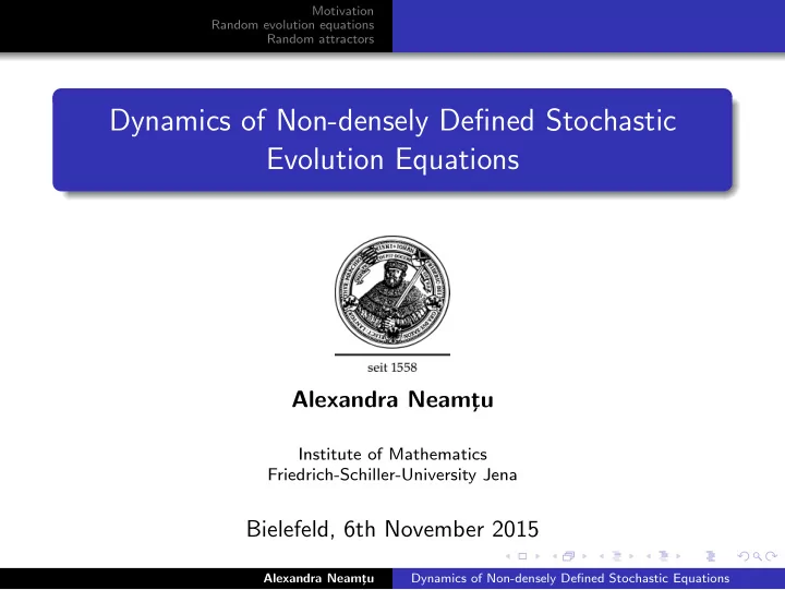
Motivation Random evolution equations Random attractors Dynamics of Non-densely Defined Stochastic Evolution Equations Alexandra Neamt ¸u Institute of Mathematics Friedrich-Schiller-University Jena Bielefeld, 6th November 2015 Alexandra Neamt ¸u Dynamics of Non-densely Defined Stochastic Equations

Motivation Random evolution equations Random attractors Motivation 1 Alexandra Neamt ¸u Dynamics of Non-densely Defined Stochastic Equations

Motivation Random evolution equations Random attractors Motivation 1 Random evolution equations 2 Alexandra Neamt ¸u Dynamics of Non-densely Defined Stochastic Equations

Motivation Random evolution equations Random attractors Motivation 1 Random evolution equations 2 Random attractors 3 Alexandra Neamt ¸u Dynamics of Non-densely Defined Stochastic Equations

Motivation Random evolution equations Random attractors SDE : � dU ( t ) = ( AU ( t ) + F ( U ( t ))) dt + dW ( t ) , t ∈ [0 , T ] (1.1) U (0) = U 0 . RDE : � dv ( t ) = Av ( t ) + F ( ω, v ( t )) , t ∈ [0 , T ] dt (1.2) v (0) = v 0 . Dynamics 1 random attractors; 2 invariant manifolds. Alexandra Neamt ¸u Dynamics of Non-densely Defined Stochastic Equations

Motivation Random evolution equations Random attractors SDE : � dU ( t ) = ( AU ( t ) + F ( U ( t ))) dt + dW ( t ) , t ∈ [0 , T ] (1.1) U (0) = U 0 . RDE : � dv ( t ) = Av ( t ) + F ( ω, v ( t )) , t ∈ [0 , T ] dt (1.2) v (0) = v 0 . Dynamics 1 random attractors; 2 invariant manifolds. Here: A is a non-densely defined linear operator: NO C 0 -semigroup! Alexandra Neamt ¸u Dynamics of Non-densely Defined Stochastic Equations

Motivation Random evolution equations Random attractors Example: Deterministic case Age-structured models in population dynamics [P. Magal and S. Ruan (2009)] ∂ t v ( t , a ) + ∂ a v ( t , a ) = − µ v ( t , a ) , t > 0 , a > 0 ,  � ∞  �  � v ( t , 0) = f β ( a ) v ( t , a ) da 0   v (0 , · ) = v 0 ( · ) ∈ L 1 (0 , ∞ ) . Ricker type birth function: f ( x ) = xe − bx , x ∈ R and b > 0. Alexandra Neamt ¸u Dynamics of Non-densely Defined Stochastic Equations

Motivation Random evolution equations Random attractors Example: Deterministic case Age-structured models in population dynamics [P. Magal and S. Ruan (2009)] ∂ t v ( t , a ) + ∂ a v ( t , a ) = − µ v ( t , a ) , t > 0 , a > 0 ,  � ∞  �  � v ( t , 0) = f β ( a ) v ( t , a ) da 0   v (0 , · ) = v 0 ( · ) ∈ L 1 (0 , ∞ ) . Ricker type birth function: f ( x ) = xe − bx , x ∈ R and b > 0. 0 � � Set X = R × L 1 (0 , ∞ ) and u ( t , · ) = . v ( t , · ) � 0 − v (0) � � � with D ( A ) = { 0 } × W 1 , 1 (0 , ∞ ). A = − v ′ − µ v v   � ∞ � 0 � � �  f β ( a ) v ( a ) da F : { 0 } × L 1 (0 , ∞ ) → X , F  . = v 0 0 Alexandra Neamt ¸u Dynamics of Non-densely Defined Stochastic Equations

Motivation Random evolution equations Random attractors Abstract Cauchy-Problem One obtains du = Au + F ( u ) , u (0) = u 0 ∈ D ( A ) . (1.3) Note that D ( A ) = { 0 } × L 1 (0 , ∞ ) � = X . Alexandra Neamt ¸u Dynamics of Non-densely Defined Stochastic Equations

Motivation Random evolution equations Random attractors Abstract Cauchy-Problem One obtains du = Au + F ( u ) , u (0) = u 0 ∈ D ( A ) . (1.3) Note that D ( A ) = { 0 } × L 1 (0 , ∞ ) � = X . G. Da Prato and E. Sinestrari, Differential operators with non-dense domain , Ann. Scuola. Norm. Sup. Pisa Cl. Sci 14 (1987), 285-344; Z. Liu, P. Magal and S. Ruan, Hopf bifurcation for nondensely defined Cauchy problems , Z. Angew. Math. Phys. 62 (2011), 191-222; P. Magal, S. Ruan, On semilinear Cauchy problems with nondense domain , Adv. Diff. Eq. 14 (2009), 1041-1084; H. R. Thieme, Integrated semigroups and integrated solutions to abstract Cauchy problems , J. Math. Anal. Appl. 152 (1990), 416-447. Alexandra Neamt ¸u Dynamics of Non-densely Defined Stochastic Equations

Motivation Random evolution equations Random attractors Preliminaries Definition Let θ : R × Ω → Ω be a family of P -preserving transformations having following properties: 1 the mapping ( t , ω ) �→ θ t ω is ( B ( R ) ⊗ F , F )-measurable; 2 θ 0 = Id Ω ; 3 θ t + s = θ t ◦ θ s for all t , s , ∈ R . Then the quadrupel (Ω , F , P , ( θ t ) t ∈ R ) is called a metric dynamical system. Definition A linear random dynamical system is a mapping ϕ : R + × Ω × X → X , ( t , ω, x ) �→ ϕ ( t , ω, x ) , ϕ is ( B ( R + ) ⊗ F ⊗ B ( X ), B ( X ))-measurable; 1 2 ϕ (0 , ω, · ) = Id X for all ω ∈ Ω; 3 the cocycle property: ϕ ( t + s , ω, x ) = ϕ ( t , θ s ω, ϕ ( s , ω, x )) , for all x ∈ X , s , t ∈ R + , ω ∈ Ω; for each ω ∈ Ω and t ∈ R + , [ X ∋ x �→ ϕ ( t , ω, x ) ∈ X ] ∈ L ( X ). 4 Alexandra Neamt ¸u Dynamics of Non-densely Defined Stochastic Equations

Motivation Random evolution equations Random attractors RDE Let X be a separable Banach space and X 0 := D ( A ); u ′ ( t ) = Au ( t ) + F ( θ t ω, u ( t )) , u (0) = u 0 ∈ X 0 . (2.1) Definition A family of linear bounded operators ( S ( t )) t ≥ 0 is called an integrated semigroup if S (0) = 0; 1 t �→ S ( t ) is strongly continuous; 2 s � S ( s ) S ( t ) = ( S ( r + t ) − S ( r )) dr , t , s ≥ 0. 3 0 Examples: t � S ( t ) = T ( s ) ds where ( T ( t )) t ≥ 0 is a C 0 -semigroup; 1 0 Au = i ∆ u generates an integrated semigroup in L p ( R n ) for p � = 2. 2 Alexandra Neamt ¸u Dynamics of Non-densely Defined Stochastic Equations

Motivation Random evolution equations Random attractors Definition A continuous map u ∈ C ([0 , T ]; X ) is an integrated solution of (2.1) if t � u ( s ) ds ∈ D ( A ) , t ∈ [0 , T ]; 1 0 t t � � u ( t ) = u 0 + A u ( s ) ds + F ( θ s ω, u ( s , ω, u 0 )) ds , t ∈ [0 , T ]. 2 0 0 Assumptions : M � � ( λ I − A ) − k � (a) L ( X 0 ) ≤ ( λ − ω A ) k , for all λ > ω A and all k ≥ 1; � � � λ →∞ ( λ I − A ) − 1 x = 0 , for all x ∈ X . (b) lim A 0 = A on D ( A 0 ) = { x ∈ D ( A ) : Ax ∈ X 0 } generates a C 0 -semigroup ( T ( t )) t ≥ 0 on X 0 ; A generates an integrated semigroup ( S ( t )) t ≥ 0 on X . Alexandra Neamt ¸u Dynamics of Non-densely Defined Stochastic Equations

Motivation Random evolution equations Random attractors Variation of constants ( λ I − A ) − 1 : X → X 0 and λ →∞ λ ( λ I − A ) − 1 x = x , for x ∈ X 0 . lim Equation on X 0 : ( λ I − A ) − 1 du ( t ) = A 0 ( λ I − A ) − 1 u ( t ) dt + ( λ I − A ) − 1 F ( θ t ω, u ( t )) dt , t � ( λ I − A ) − 1 u ( t ) = T ( t )( λ I − A ) − 1 u 0 + T ( t − s )( λ I − A ) − 1 F ( θ s ω, u ( s )) ds . 0 Theorem Equation (2.1) possesses a unique global integrated solution t � T ( t − s ) λ ( λ I − A ) − 1 F ( θ s ω, u ( s , ω, u 0 )) ds . u ( t , ω, u 0 ) = T ( t ) u 0 + lim λ →∞ 0 (2.2) Alexandra Neamt ¸u Dynamics of Non-densely Defined Stochastic Equations

Motivation Random evolution equations Random attractors Special case Consider du ( t ) = ( Au ( t ) + f ( u ( t ))) dt + σ dW ( t ) , u (0) = u 0 ∈ D ( A ) , σ ∈ D ( A ) . (2.3) 0 � e s ω ( s ) ds Ornstein-Uhlenbeck process: dz = zdt + dW , z ( ω ) = − −∞ 0 e s ω ( t + s ) ds + ω ( t ) , t ∈ R . � ( t , ω ) �→ z ( θ t ω ): z ( θ t ω ) = − −∞ Transformation: x ( t ) = u ( t ) − z ( θ t ω ). x ′ ( t ) = Ax ( t ) + F ( θ t ω, x ( t )) , Equation (2.3) becomes: F ( θ t ω, x ( t )) = f ( x ( t ) + z ( θ t ω )) + Az ( θ t ω ) + z ( θ t ω ) . Alexandra Neamt ¸u Dynamics of Non-densely Defined Stochastic Equations

Motivation Random evolution equations Random attractors The parabolic case Assumptions: A 0 generates an analytic semigroup, B ∈ γ ( H ; X 0 ) and W is an H -cylindrical Wiener process. dU ( t ) = ( AU ( t ) + F ( U ( t ))) dt + BdW ( t ) v ( t ) = U ( t ) − Z ( θ t ω ) dv ( t ) = Av ( t ) dt + F ( v ( t ) + Z ( θ t ω )) dt . Infinite dimensional noise: L p ( R )-valued Brownian motion: formally ∞ ∞ � � W ( t ) = g k ( x ) w k ( t ) = W H ( t ) e k Be k . k =1 k =1 ( g k ) k ≥ 1 ∈ L p ( R , l 2 ) define Bh := � [ h , e k ] g k , h ∈ l 2 and ( e k ) k ≥ 1 ONB in l 2 . k ≥ 1 2 p � p � � � � � � � � � E γ k Be k L p ( R ) � p E γ k Be k L p ( R ) = E γ k g k ( x ) dx � � � � � � � � � � � � k ≥ 1 k ≥ 1 k ≥ 1 R p   2 � � | g k ( x ) | 2 ≤ dx < ∞ .  k ≥ 1 R Alexandra Neamt ¸u Dynamics of Non-densely Defined Stochastic Equations